Page 188 - Introduction to Statistical Pattern Recognition

170 Introduction to Statistical Pattern Recognition

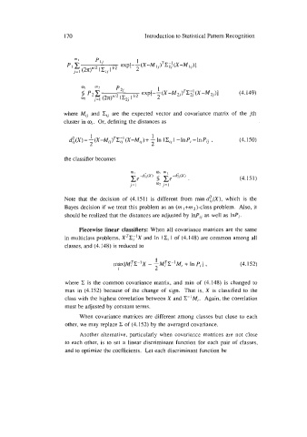
(4.149)

where Mij and Zjj are the expected vector and covariance matrix of the jth
cluster in mi. Or, defining the distances as

1 1
d*.(x) = -(x-M..)~c:' (x-M..) + - In I C, I -In P; -In pij , (4.150)
2 'J IJ 2
the classifier becomes

(4.151)

Note that the decision of (4.151) is different from min da(X), which is the
Bayes decision if we treat this problem as an (rn I+m2)-class problem. Also, it
should be realized that the distances are adjusted by lnP, as well as lnPi.

Piecewise linear classifiers: When all covariance matrices are the same
in multiclass problems, XTXT1X and In I Ci I of (4.148) are common among all
classes, and (4.148) is reduced to

where C is the common covariance matrix, and min of (4.148) is changed to
max in (4.152) because of the change of sign. That is, X is classified to the
class with the highest correlation between X and Z-'Mj. Again, the correlation
must be adjusted by constant terms.
When covariance matrices are different among classes but close to each
other, we may replace of (4.152) by the averaged covariance.
Another alternative, particularly when covariance matrices are not close
to each other, is to set a linear discriminant function for each pair of classes,
and to optimize the coefficients. Let each discriminant function be