Page 189 - Introduction to Statistical Pattern Recognition

4 Parametric Classifiers 171

(i,j = 1,. . . ,L: i # j) . (4.153)
hjj(X) = v;x + vjjo
The signs of Vij are selected such that the distribution of oj is located on the
positive side of hij(X) and pi on the negative side. Therefore,

hij(X) = +(X) . (4.154)

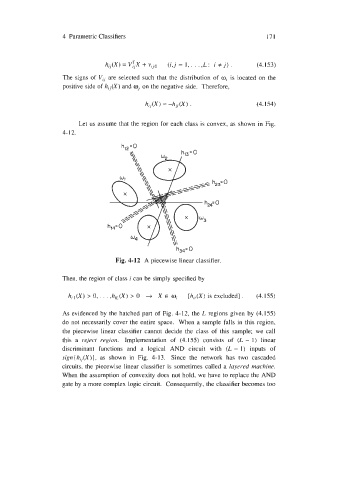
Let us assume that the region for each class is convex, as shown in Fig.
4- 12.

Fig. 4-12 A piecewise linear classifier.

Then, the region of class i can be simply specified by

.
hil(X) > 0,. . ,hjL(X) > 0 -+ X E mi [hii(X) is excluded] . (4.155)
As evidenced by the hatched part of Fig. 4-12, the L regions given by (4.155)
do not necessarily cover the entire space. When a sample falls in this region,
the piecewise linear classifier cannot decide the class of this sample; we call
this a reject region. Implementation of (4.155) consists of (L - 1) linear
discriminant functions and a logical AND circuit with (L - 1) inputs of
sign{hij(X)), as shown in Fig. 4-13. Since the network has two cascaded
circuits, the piecewise linear classifier is sometimes called a layered machine.
When the assumption of convexity does not hold, we have to replace the AND
gate by a more complex logic circuit. Consequently, the classifier becomes too