Page 267 - Introduction to Statistical Pattern Recognition

5 Parameter Estimation 249

ignored. Cov-..{yy),yf) J may be approximated by using the first term only of
(5.178). Again, using (5.184),

COV- ( 7:),7f) } = Ex ( 7y)yy) ] - E* ( y:' ]E. { yf ) }

1
=-sisn(h(X:"))sj~n(~(X1')))E { Awy)Awf) }-E.. { y:' ]E* (yf' ]
4
(5.186)

where E(Aw:"Aw~)] =-I/NP for j +k by (5.166), and E*(yy)]E*{yf)} is
proportional to I/Nf by (5.180) and therefore can be ignored.

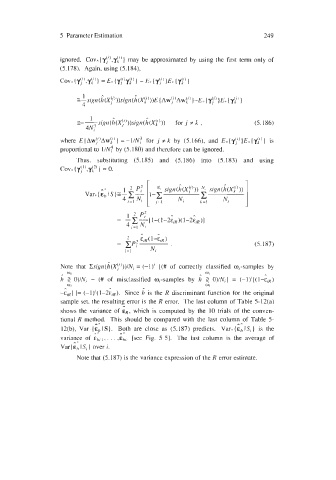
Thus, substituting (5.185) and (5.186) into (5.183) and using
covx (y:",yp J = 0,

r 1

(5.187)
i=I [Vi

Note that Csign(L(X,Y'))/Ni = (-1)' [(# of correctly classified mi-samples by
.. 01 ,. 01
h >< O)/N, - (# of misclassified mi-samples by h >< O)/Ni] = (-l)'[(1-qR)
W? ,. W?
-eiR] ]= (-l)1(1-2~lR). Since h is the R discriminant function for the original
,.
sample set, the resulting error is the R error. The last column of Table 5-12(a)
shows the variance of E~. which is computed by the 10 trials of the conven-
tional R method. This should be compared with the last column of Table 5-
r*
12(b), Var,($IS). Both are close as (5.187) predicts. Var,{&,,ISi] is the
..*
variance of . . . [see Fig. 5-51. The last column is the average of
AX
Var( E,, I Si } over i.
Note that (5.187) is the variance expression of the R error estimate.