Page 294 - Introduction to Statistical Pattern Recognition

276 Introduction to Statistical Pattern Recognition

to B. Also, note that the same optimal metric is obtained by minimizing MSE*
of (6.98), and thus the metric is optimal locally as well as globally.

Normal example: The optimal k for a normal distribution can be com-
puted easily. For a normal distribution with zero expected vector and identity
covariance matrix,

(6.104)

(6.105)

Substituting (6.104) and (6.105) into (6. loo), and noting that the optimal
metric A is I in this case,
I;" 4

k* = N ll+4 . (6.106)
-

4 1 1 1 1 1 1
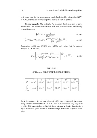
TABLE 6-2

OPTIMAL k FOR NORMAL DISTRIBUTIONS

16
8
32
64
128
0.75 N 'I2 0.94N 0.62 N 0.34 N 'I9 0.17 N "I7 0.09 N
for 4.4~10 1.5~10' 3.4~10~ 3.2~10'" 9.2~10~~ 3.8~10~~
k*=5

Table 6-2 shows k* for various values of n [5]. Also, Table 6-2 shows how
many samples are needed for k* to be 5. Note that N becomes very large after
n = 16. This suggests how difficult it is to estimate a density function in a
high-dimensional space, unless an extremely large number of samples is avail-
able.