Page 30 - Introduction to Statistical Pattern Recognition

12 Introduction to Statistical Pattern Recognition

where Pr(A) is the probability of an event A. For convenience, we often write
(2.2) as
P(X) = Pr(X 5x1 . (2.3)

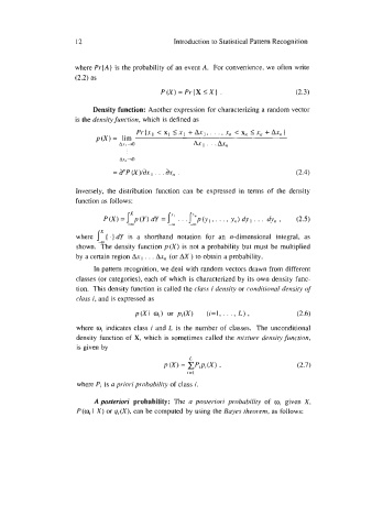
Density function: Another expression for characterizing a random vector
is the density function, which is defined as
Pr(xl <xl <xl+Ax,, ..., ~~<x,~~x,,+Ax~~)
p(X) = lim
Av I +O AX^ . . .AX,,

Inversely, the distribution function can be expressed in terms of the density
function as follows:
P(X)=j p(Y)dY =I”’. 1 Yr,) dY I ’ .
-
X
.
.-ca
where ( .) dY is a shorthand notation for an n-dimensional integral, as
shown. -?he density function p (X) is not a probability but must be multiplied
by a certain region Ax I . . . Axrl (or AX ) to obtain a probability.
In pattern recognition, we deal with random vectors drawn from different
classes (or categories), each of which is characterized by its own density func-
tion. This density function is called the class i density or conditional density of
class i, and is expressed as

p(X I 0,) or p,(X) (i=l, . . . , L) , (2.6)
where 0, indicates class i and L is the number of classes. The unconditional
density function of X, which is sometimes called the mixture densiry function,
is given by

where Pi is a priori probability of class i.
Aposteriori probability: The a posteriori probability of mi given X,
P(wj X) or qi(X), can be computed by using the Bayes theorem, as follows:
I