Page 300 - Introduction to Statistical Pattern Recognition

282 Introduction to Statistical Pattern Recognition

where use has been made of T(x+l) =xT(x). Measuring the left-hand side
from the given data set and solving (6.1 15) for n, we can obtain the local
dimensionality [18],[21].
In succeeding chapters, we will discuss the effect of dimensionality in
various nonparametric operations. The dimensionality is the most important
parameter in determining nonparametric properties as was already seen in
E(dFN(X)) of (6.108). However, note that the dimensionality in non-
parametric operations automatically means the intrinsic or local dimensionality.
Without realizing this fact, readers may often find a discrepancy between
theoretical and experimental results.

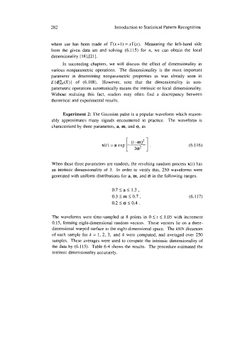
Experiment 2: The Gaussian pulse is a popular waveform which reason-
ably approximates many signals encountered in practice. The waveform is
characterized by three parameters, a, m, and Q, as

x(t) = a exp 1-91 . (6.1 16)

When these three parameters are random, the resulting random process x(t) has
an intrinsic dimensionality of 3. In order to verify this, 250 waveforms were
generated with uniform distributions for a, rn, and (T in the following ranges.

0.7 5 a I 1.3 ,
0.3 I 50.7 , (6.1 17)
m
0.2 5 o 10.4 .

The waveforms were time-sampled at 8 points in 0 S r I 1.05 with increment
0.15, forming eight-dimensional random vectors. These vectors lie on a three-
dimensional warped surface in the eight-dimensional space. The kNN distances
of each sample for k = I, 2, 3, and 4 were computed, and averaged over 250
samples. These averages were used to compute the intrinsic dimensionality of
the data by (6.1 15). Table 6-4 shows the results. The procedure estimated the
intrinsic dimensionality accurately.