Page 36 - Introduction to Statistical Pattern Recognition

18 Introduction to Statistical Pattern Recognition

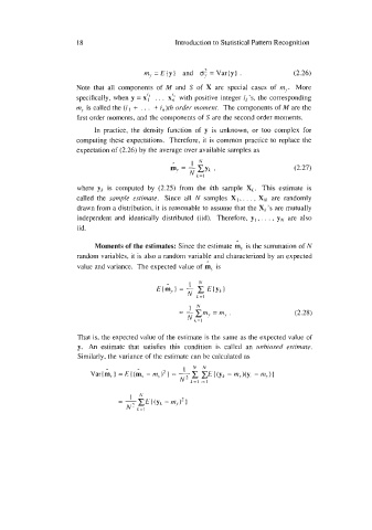
m, =E{y} and 0; =Var(y) . (2.26)
Note that all components of M and S of X are special cases of m,. More
specifically, when y = x:’ . . . x: with positive integer ih’s, the corresponding
m, is called the (i I + . . . + i,,)th order. moment. The components of M are the
first order moments, and the components of S are the second order moments.

In practice, the density function of y is unknown, or too complex for
computing these expectations. Therefore, it is common practice to replace the
expectation of (2.26) by the average over available samples as
,. lN
m\ =-CY!, , (2.27)
h=l
where yh is computed by (2.25) from the kth sample x,. This estimate is
called the sample estimate. Since all N samples XI,. . . , XN are randomly
drawn from a distribution, it is reasonable to assume that the Xk’s are mutually
independent and identically distributed (iid). Therefore, yI , . . . , yN are also
iid.

Moments of the estimates: Since the estimate m, is the summation of N
random variables, it is also a random variable and characterized by an expected
value and variance. The expected value of m, is

lh
(2.28)

That is, the expected value of the estimate is the same as the expected value of
y. An estimate that satisfies this condition is called an unhiased estimate.
Similarly, the variance of the estimate can be calculated as