Page 38 - Introduction to Statistical Pattern Recognition

20 Introduction to Statistical Pattern Recognition

A A
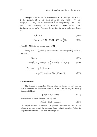
Example 1: For mi, the ith component of M, the corresponding y is xi.
If the moments of xi are given as .!?(xi} =mi, Var(xi} =of, and
,.
Cov(xj,xi} =pijojaj, then the moments of mi are computed by (2.28), (2.29),
and (2.30), resulting in E { mi 1 = mi, Var( mi } = o?/N, and
* A
Cov( mi,mj) = pijaioj/N. They may be rewritten in vector and matrix forms
as

E(MJ =M, (2.33)
1
Cov{M) =E((M-M)(M-M)T) =-E, (2.34)
N

where Cov( M} is the covariance matrix of M.
,.
A
Example 2: For sjj, the i, j component of S, the corresponding y is xix,;.
Therefore,

A
E(Sjj} = Sjj , (2.35)
A
Var(sij} = -Var(xixj} = 1 -[[E{xixj -E 2 (xjxj)l, (2.36)
1
}
2
2
N N
A,. 1
Cov( s;j,spt ) = -Cov( x;xj.xpx, )
N
= -[E{xixjxkx;} -E(xixj}E{XkX;Il. (2.37)
1
N
Central Moments

The situation is somewhat different when we discuss central moments
such as variances and covariance matrices. If we could define y for the i, j
component of as
y = (xi - mi)(xi - mj) (2.38)

with the given expected values mi and mi, then
A
E(m,} = E{y} = pijoioj . (2.39)
The sample estimate is unbiased. In practice, however, mi and mi are
unknown, and they should be estimated from available samples. When the
sample means are used, (2.38) must be changed to