Page 78 - Introduction to Statistical Pattern Recognition

60 Introduction to Statistical Pattern Recognition

E2 = yph(h lq)dh = . (3.33)
-0
However, an analytical solution is not possible in general. So, we must find p
experimentally or numerically. Since ph(h 102) 2 0, c2 of (3.33) is a mono-
tonic function of p, and increases as p increases. Therefore, after calculating
E~’S for several p’s, we can find the p which gives a specified as c2.

Example 4: Let us consider two-dimensional normal distributions with
MI = [-l,0IT, M2 = [+1,0]‘, XI = X2 = I, and PI = P2 = 0.5. Then, from
(3.12) and (3.31), the decision boundary can be expressed by
LI

h (X) = { [+1 01 - [-1 01 1

(3.34)

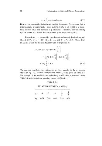
The decision boundaries for various p’s are lines parallel to the x2-axis, as
shown in Fig. 3-3, and the corresponding errors EZ’S are given in Table 3-1.
For example, if we would like to maintain e2 = 0.09, then p becomes 2 from
Table 3-1, and the decision boundary passes (-0.34) of x
TABLE 3-1

RELATION BETWEEN AND ~2

1
1
p: 4 2 - -
l 2 4
~2: 0.04 0.09 0.16 0.25 0.38