Page 83 - Introduction to Statistical Pattern Recognition

3 Hypothesis Testing 65

(3.42)

That is, if @-'(E,) and are used as the x- and y-axes, we have a

h

E* E,
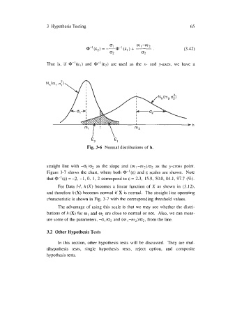
Fig. 3-6 Normal distributions of h.

straight line with -o1/o2 as the slope and (mI-rn2)/02 as the y-cross point.
Figure 3-7 shows the chart, where both @-'(E) and E scales are shown. Note
that @-'(E) =-2, -1, 0, 1, 2 correspond to E = 2.3, 15.9, 50.0, 84.1, 97.7 (%).
For Data 1-1, h (X) becomes a linear function of X as shown in (3.12),
and therefore h (X) becomes normal if X is normal. The straight line operating
characteristic is shown in Fig. 3-7 with the corresponding threshold values.
The advantage of using this scale is that we may see whether the distri-
butions of h (X) for a, and w2 are close to normal or not. Also, we can meas-
ure some of the parameters, -01/02 and (rn I-rn2)/02, from the line.

3.2 Other Hypothesis Tests

In this section, other hypothesis tests will be discussed. They are mul-
tihypothesis tests, single hypothesis tests, reject option, and composite
hypothesis tests.