Page 88 - Introduction to Statistical Pattern Recognition

70 Introduction to Statistical Pattern Recognition

L
yy

-r
I
0 n
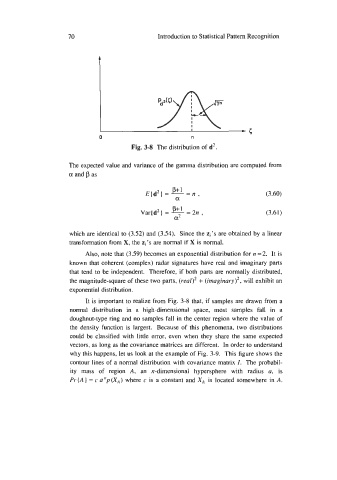
Fig. 3-8 The distribution of d2.

The expected value and variance of the gamma distribution are computed from
a and as

(3.60)

Var(d2] = = 2n , (3.61)
a2
which are identical to (352) and (3.54). Since the zi’s are obtained by a linear
transformation from X, the zi’s are normal if X is normal.
Also, note that (3.59) becomes an exponential distribution for n =2. It is
known that coherent (complex) radar signatures have real and imaginary parts
that tend to be independent. Therefore, if both parts are normally distributed,
the magnitude-square of these two parts, (real)2 + will exhibit an
exponential distribution.
It is important to realize from Fig. 3-8 that, if samples are drawn from a
normal distribution in a high-dimensional space, most samples fall in a
doughnut-type ring and no samples fall in the center region where the value of
the density function is largest. Because of this phenomena, two distributions
could be classified with little error, even when they share the same expected
vectors, as long as the covariance matrices are different. In order to understand
why this happens, let us look at the example of Fig. 3-9. This figure shows the
contour lines of a normal distribution with covariance matrix I. The probabil-
ity mass of region A, an n-dimensional hypersphere with radius a, is
Pr(A } = c ~ ‘ (XA) where c is a constant and XA is located somewhere in A.
p
~