Page 90 - Introduction to Statistical Pattern Recognition

72 Introduction to Statistical Pattern Recognition

(3.63)

Likewise, the variance can be computed as

(3.64)
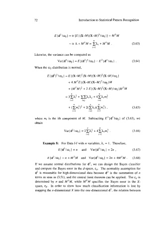
When the w2-distribution is normal,

E { (d2)2 1% ] = E ((X-M)7(X-M)(X-M)T(X-M) I O, )
+ 4 M'E ( (X-M>(X-Mf 1% }M

+ (MTM)2 + 2 E{ (X-M)T(X-M) I02 )MTM
n n
+
+
= 3~h? ~~hihj 4zhim;
i=l itj i=l
(3.65)

where mi is the ith component of M. Subtracting E2(d21q) of (3.63), we
obtain

(3.66)

Example 8: For Data I-I with n variables, hi = 1. Therefore,
E(d210,) =n and Var{d2101] =2n, (3.67)

E(d21w) =n +M'M and Var(d2102] =2n +4M7M. (3.68)

If we assume normal distributions for d2, we can design the Bayes classifier
and compute the Bayes error in the d-space, E~. The normality assumption for
d2 is reasonable for high-dimensional data because d2 is the summation of n
terms as seen in (3.51), and the central limit theorem can be applied. The &d is
determined by n and MTM, while MTM specifies the Bayes error in the X-
space, In order to show how much classification information is lost by
mapping the n-dimensional X into the one-dimensional d2, the relation between