Page 92 - Introduction to Statistical Pattern Recognition

74 Introduction to Statistical Pattern Recognition

I
P, =j kl(l-ul)kl-’(1-*2)kzdUI (3.69)
,
0
where

u;(f) = [pd’(< 1 mi)d< (3.70)
andpdz((lmi) is the density function of < = d2 for ai. As seen in (3.70), u&)
is the probability of a sample from ai falling in 0 I < < t. Thus, u (t) = l--~~
I
in
and u2(r) =E~ the d-space when the threshold is chosen at d2 = f. In (3.69),
du,, (l-uIf’-’, and (1-u2$’ represent the probability of one of kl ol-
samples falling in f 5 < < r +At, kl-1 of al-samples falling in f +At I
< < 00, and all k2 m2-samples falling in t + Ar I & < 00 respectively. The pro-
duct of these three gives the probability of the combined event. Since the
acquisition of any one of the kl ol-samples is a correct classification, the pro-
bability is multiplied by k I. The integration is taken with respect to f from 0
to 00, that is, with respect to u I from 0 to 1.

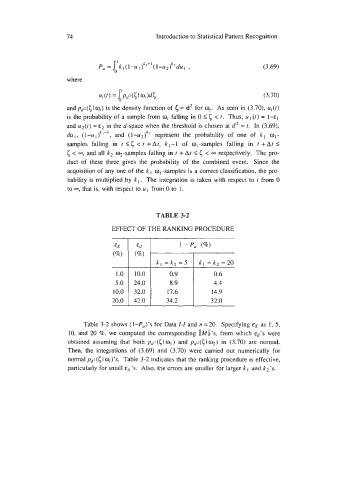
TABLE 3-2

Ed 1 -Pa (%)
(%o) (%)
k1 =k2 =5 k1 =k2=20
1.0 10.0 0.9 0.6
5.0 24.0 8.9 4.4
10.0 32.0 17.6 14.9
20.0 42.0 34.2 32.0

Table 3-2 shows (l-Po)’s for Data I-I and n =20. Specifying &x as 1, 5,
10, and 20 %, we computed the corresponding llkfll’s, from which E~’S were
obtained assuming that both pc,l((I~l) and pdz(<lw) in (3.70) are normal.
Then, the integrations of (3.69) and (3.70) were carried out numerically for
normal pd’(< I wj)’s. Table 3-2 indicates that the ranking procedure is effective,
particularly for small E~’s. Also, the errors are smaller for larger k I and k2 ’s.