Page 298 - Materials Chemistry, Second Edition

284 R.K. Rosenbaum et al.

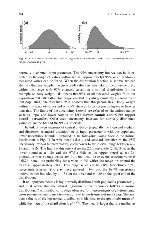
Fig. 11.7 a Normal distribution and b log-normal distribution with 95% uncertainty interval
ranges shaded in grey

normally distributed input parameter. This 95% uncertainty interval can be inter-
preted as the range of values within which (approximately) 95% of all randomly
measured values can be found. When the distribution function is known, we can
also say that any sampled (or measured) value one may take in the future will fall
within this range with 95% chances. Assuming a normal distribution for our
example on body weight, this means that 95% of all measured weights from our
population will fall within this range and that if picking randomly a person from
that population, one will have 95% chances that this person has a body weight
within this range of values and only 5% chances to pick a person lighter or heavier
than that. The limits of the uncertainty interval are referred to via various names
such as upper and lower bounds or 2.5th (lower bound) and 97.5th (upper
bound) percentiles. Other used uncertainty intervals for normally distributed
variables are the 68 and the 99.7% intervals.
The link between measures of central tendency (especially the mean and median)
and dispersion (standard deviation) of an input parameter x with the upper and
lower uncertainty bounds is detailed in the following. Going back to the normal
distribution in Fig. 11.7a with mean value l and standard deviation r, the 95%
uncertainty interval (approximately) corresponds to the interval range between l
2r and l þ 2r. The limits of this interval are the 2.5th percentile (2.5th %ile) as the
lower bound at l 2r and the 97.5th %ile as the upper bound at l þ 2r.
Integrating over a range within r from the mean value l, the resulting value is
0.6826; hence, the probability for a value to fall within the range r around the
mean is approximately 68%. This range is called the 68% (sometimes 65%)
uncertainty interval. You may have guessed it by now, the 99.7% uncertainty
interval is then bounded by l 3r on the lower and l þ 3r on the upper end of the
distribution.
If an input parameter x is log-normally distributed with population parameters l
and r, it means that the natural logarithm of the parameter follows a normal
distribution. This distribution is often observed for measurements of environmental
input parameters and hence frequently used in environmental modelling. The me-
l
dian value m of the log-normal distribution is identical to the geometric mean e ,
2
while the mean of the distribution is e l þ r =2 . The mean is larger than the median as