Page 146 - A First Course In Stochastic Models

138 DISCRETE-TIME MARKOV CHAINS

(a) Modify the one-step transition probabilities of the Markov chain {X n } describing the
number of messages in the buffer at the end of the time slots.
(K)
(b) Denoting by {π , j = 0, 1, . . . , K} the equilibrium distribution of the Markov
j
chain, argue that the long-run fraction of messages lost is
 
c−1 K
1 (K) (K)
π loss (K) =  λ − jπ j − c π j  .
λ
j=1 j=c
(Hint: the sum of the average number of messages lost per time unit and the average number
of messages transmitted per time unit equals λ.)
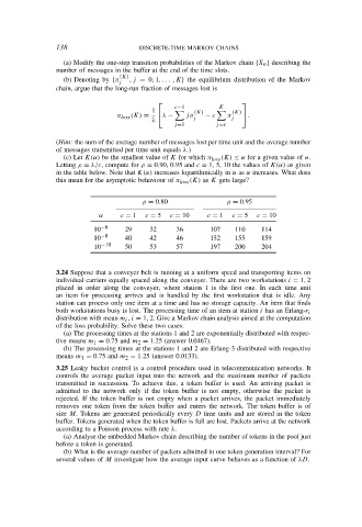
(c) Let K(α) be the smallest value of K for which π loss (K) ≤ α for a given value of α.
Letting ρ = λ/c, compute for ρ = 0.90, 0.95 and c = 1, 5, 10 the values of K(α) as given
in the table below. Note that K(α) increases logarithmically in α as α increases. What does
this mean for the asymptotic behaviour of π loss (K) as K gets large?

ρ = 0.80 ρ = 0.95
α c = 1 c = 5 c = 10 c = 1 c = 5 c = 10
10 −6 29 32 36 107 110 114
10 −8 40 42 46 152 155 159
10 −10 50 53 57 197 200 204

3.24 Suppose that a conveyer belt is running at a uniform speed and transporting items on
individual carriers equally spaced along the conveyer. There are two workstations i = 1, 2
placed in order along the conveyer, where station 1 is the first one. In each time unit
an item for processing arrives and is handled by the first workstation that is idle. Any
station can process only one item at a time and has no storage capacity. An item that finds
both workstations busy is lost. The processing time of an item at station i has an Erlang-r i
distribution with mean m i , i = 1, 2. Give a Markov chain analysis aimed at the computation
of the loss probability. Solve these two cases:
(a) The processing times at the stations 1 and 2 are exponentially distributed with respec-
tive means m 1 = 0.75 and m 2 = 1.25 (answer 0.0467).
(b) The processing times at the stations 1 and 2 are Erlang-3 distributed with respective
means m 1 = 0.75 and m 2 = 1.25 (answer 0.0133).
3.25 Leaky bucket control is a control procedure used in telecommunication networks. It
controls the average packet input into the network and the maximum number of packets
transmitted in succession. To achieve this, a token buffer is used. An arriving packet is
admitted to the network only if the token buffer is not empty, otherwise the packet is
rejected. If the token buffer is not empty when a packet arrives, the packet immediately
removes one token from the token buffer and enters the network. The token buffer is of
size M. Tokens are generated periodically every D time units and are stored in the token
buffer. Tokens generated when the token buffer is full are lost. Packets arrive at the network
according to a Poisson process with rate λ.
(a) Analyse the embedded Markov chain describing the number of tokens in the pool just
before a token is generated.
(b) What is the average number of packets admitted in one token generation interval? For
several values of M investigate how the average input curve behaves as a function of λD.