Page 155 - A First Course In Stochastic Models

148 CONTINUOUS-TIME MARKOV CHAINS

l l l
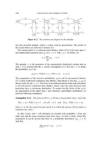
0, 1 1, 1 • • • i − 1, 1 i, 1 i + 1, 1 • • •

m m m
d b d b d b d b
l l
• • • i + 1, 0 • • •
i − 1, 0 i, 0
1, 0
Figure 4.1.2 The transition rate diagram for the unloader

into this powerful method, which is widely used by practitioners. The proofs of
the results below are deferred to Section 4.3.
The starting point is a continuous-time Markov chain {X(t)} with state space I
and infinitesimal transition rates q ij for i, j ∈ I with j = i. As before, let

ν i = q ij , i ∈ I.
j =i

The quantity ν i is the parameter of the exponentially distributed sojourn time in
state i. It is assumed that the ν i satisfy Assumption 4.1.2. For any t ≥ 0, define
the probability p ij (t) by

p ij (t) = P {X(t) = j | X(0) = i}, i, j ∈ I.

The computation of the transient probabilities p ij (t) will be discussed in Section
4.5. A deep result from continuous-time Markov chain theory is that lim t→∞ p ij (t)
always exists for all i, j ∈ I. The issue of possible periodicity in the state transitions
is not relevant for continuous-time Markov chains, since the times between state
transitions have a continuous distribution. To ensure that the limits of the p ij (t)
are independent of the initial state i and constitute a probability distribution, we
need the following assumption.

Assumption 4.2.1 The process {X(t), t ≥ 0} has a regeneration state r such that
P {τ r < ∞ | X(0) = i} = 1 f or all i ∈ I and E(τ r | X(0) = r) < ∞,

where τ r is the first epoch beyond epoch 0 at which the process {X(t)} makes a
transition into state r.

In other words, state r will ultimately be reached with probability 1 from any
other state and the mean recurrence time from state r to itself is finite. Under this
assumption it can be proved that there is a probability distribution {p j , j ∈ I}
such that

lim p ij (t) = p j , j ∈ I,
t→∞