Page 195 - A First Course In Stochastic Models

188 MARKOV CHAINS AND QUEUES

independent random variables having a common exponential distribution with mean
1/µ. The service times and the arrival process are independent of each other. Let

λ
ρ = . (5.1.1)
cµ
It is assumed that ρ < 1. Rewriting this condition as λ/µ < c, the condition states
that the average amount of work offered to the servers per time unit is less than
the total service capacity. The factor ρ is called the server utilization. This model
is a basic model in queueing theory and is often called the Erlang delay model. It
is usually abbreviated as the M/M/c queue. Using continuous-time Markov chain
theory we will derive the distributions of the queue size and the delay in queue of
a customer. Let
X(t) = the number of customers present at time t

(including any customer in service). Then the stochastic process {X(t)} is a continu-
ous-time Markov chain with infinite state space I = {0, 1, . . . }. The assumption
ρ < 1 implies that the Markov chain satisfies Assumption 4.2.1 with regeneration
state 0 and thus has a unique equilibrium distribution {p j } (a formal proof is
omitted). The probability p j gives the long-run fraction of time that j customers
are present.

5.1.1 The M/M/1 Queue
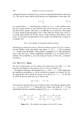
For ease of presentation, we first analyse the single-server case with c = 1. The
transition rate diagram of the process {X(t)} is given in Figure 5.1.1
Note that for each state i the transition rate q ij = 0 for j ≤ i−2. This implies that
the equilibrium probabilities p j can be recursively computed; see formula (4.2.10).
By equating the rate at which the process leaves the set {i, i + 1, . . . } to the rate
at which the process enters this set, it follows that

µp i = λp i−1 , i = 1, 2, . . . .

The recurrence equation allows for an explicit solution. Iterating the equation yields
i
p i = (λ/µ) p 0 for all i ≥ 1. Noting that this relation also holds for i = 0 and
substituting it into the normalizing equation ∞ p i = 1, we find p 0 (1−λ/µ) −1 =
i=0

l l l
0 1 • • • i − 1 i i + 1 • • •
m m m

Figure 5.1.1 The transition rate diagram for the M/M/1 queue