Page 198 - A First Course In Stochastic Models

THE ERLANG DELAY MODEL 191

l l l
0 1 • • • i − 1 i i + 1 • • •
m im (i + 1) m

l l
c − 1 c • • • j − 1 j • • •

cm cm
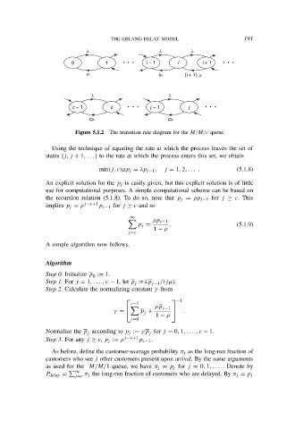
Figure 5.1.2 The transition rate diagram for the M/M/c queue

Using the technique of equating the rate at which the process leaves the set of
states {j, j + 1, . . . } to the rate at which the process enters this set, we obtain

min(j, c)µp j = λp j−1 , j = 1, 2, . . . . (5.1.8)
An explicit solution for the p j is easily given, but this explicit solution is of little
use for computational purposes. A simple computational scheme can be based on
the recursion relation (5.1.8). To do so, note that p j = ρp j−1 for j ≥ c. This
implies p j = ρ j−c+1 p c−1 for j ≥ c and so

∞
ρp c−1
p j = . (5.1.9)
1 − ρ
j=c
A simple algorithm now follows.

Algorithm

Step 0. Initialize p := 1.
0
Step 1. For j = 1, . . . , c − 1, let p := λp /(jµ).
j j−1
Step 2. Calculate the normalizing constant γ from
  −1
c−1
ρp
c−1
γ =  p +  .
j
j=0 1 − ρ
Normalize the p according to p j := γ p for j = 0, 1, . . . , c − 1.
j j
Step 3. For any j ≥ c, p j := ρ j−c+1 p c−1 .
As before, define the customer-average probability π j as the long-run fraction of
customers who see j other customers present upon arrival. By the same arguments
as used for the M/M/1 queue, we have π j = p j for j = 0, 1, . . . . Denote by

∞
P delay = j=c π j the long-run fraction of customers who are delayed. By π j = p j