Page 203 - A First Course In Stochastic Models

196 MARKOV CHAINS AND QUEUES

Note that the distribution in (5.2.1) is a truncated Poisson distribution (multiply
both the numerator and the denominator by e −λ/µ ). Denote by the customer-average
probability π i the long-run fraction of messages that find i other messages present
upon arrival. Then, by the PASTA property,

π i = p i , i = 0, 1, . . . , c.
In particular, denoting by P loss the long-run fraction of messages that are lost,
c
(λ/µ) /c!
P loss = c k . (5.2.2)
k=0 (λ/µ) /k!
This formula is called the Erlang loss formula. As said before, the formula (5.2.1)
for the time-average probabilities p j and the formula (5.2.2) for the loss probability
remain valid when the transmission time has a general distribution with mean 1/µ.
The state probabilities p j are insensitive to the form of the probability distribution
of the transmission time and require only the mean transmission time. Letting c →
∞ in (5.2.1), we get the Poisson distribution with mean λ/µ in accordance with
earlier results for the M/G/∞ queue. The insensitivity property of this infinite-
server queue was proved in Section 1.1.3.

5.2.2 The Engset Model
The Erlang loss model assumes Poisson arrivals and thus has an infinite source of
potential customers. The Engset model differs from the Erlang loss model only by
assuming a finite source of customers. There are M sources which generate service
requests for c service channels. It is assumed that M > c. A service request that is
generated when all c channels are occupied is lost. Each source is alternately on and
off. A source is off when it has a service request being served, otherwise the source
is on. A source in the on-state generates a new service request after an exponentially
distributed time (the think time) with mean 1/α. The sources act independently of
each other. The service time of a service request has an exponential distribution
with mean 1/µ and is independent of the think time. This model is called the
Engset model after Engset (1918).
We now let
X(t) = the number of occupied channels at time t.

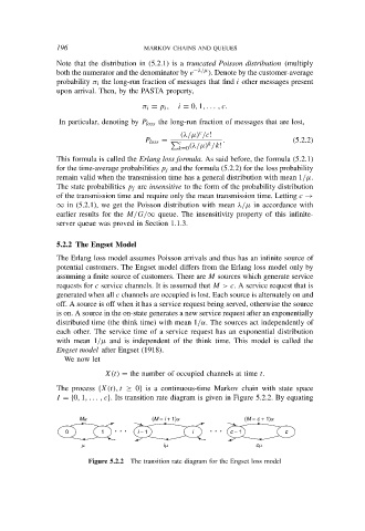
The process {X(t), t ≥ 0} is a continuous-time Markov chain with state space
I = {0, 1, . . . , c}. Its transition rate diagram is given in Figure 5.2.2. By equating

Ma (M − i + 1)a (M − c + 1)a
0 1 • • • i − 1 i • • • c − 1 c
m im cm

Figure 5.2.2 The transition rate diagram for the Engset loss model