Page 206 - A First Course In Stochastic Models

SERVICE-SYSTEM DESIGN 199

Note that R is a dimensionless quantity that gives the average amount of work
offered per time unit to the c servers. The offered load R is often expressed as R
erlangs of work. In order to ensure the existence of a steady-state regime for the
queue, it should be assumed that the service capacity c is larger than the offered
load R. Hence the assumption is made that the server utilization
R
ρ =
c
is less than 1. Note that ρ represents the long-run fraction of time a given server is
busy. In the single-server case the server utilization ρ should not be too close to 1
in order to avoid excessive waiting of the customers. A rule of thumb for practical
applications of the M/M/1 model is that the server utilization should not be much
above 0.8. A natural question is how this rule of thumb should be adjusted for the
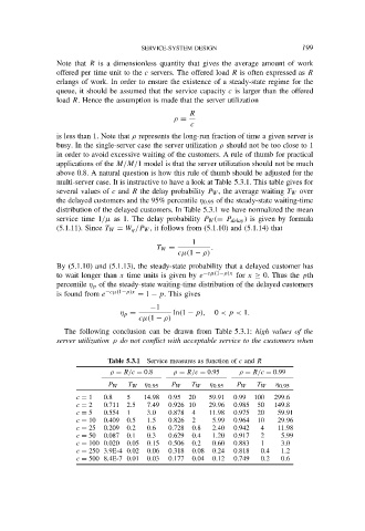
multi-server case. It is instructive to have a look at Table 5.3.1. This table gives for
several values of c and R the delay probability P W , the average waiting T W over
the delayed customers and the 95% percentile η 0.95 of the steady-state waiting-time
distribution of the delayed customers. In Table 5.3.1 we have normalized the mean
service time 1/µ as 1. The delay probability P W (= P delay ) is given by formula
(5.1.11). Since T W = W q /P W , it follows from (5.1.10) and (5.1.14) that

1
T W = .
cµ(1 − ρ)
By (5.1.10) and (5.1.13), the steady-state probability that a delayed customer has
to wait longer than x time units is given by e −cµ(1−ρ)x for x ≥ 0. Thus the pth
percentile η p of the steady-state waiting-time distribution of the delayed customers
is found from e −cµ(1−ρ)x = 1 − p. This gives
−1
η p = ln(1 − p), 0 < p < 1.
cµ(1 − ρ)
The following conclusion can be drawn from Table 5.3.1: high values of the
server utilization ρ do not conflict with acceptable service to the customers when

Table 5.3.1 Service measures as function of c and R
ρ = R/c = 0.8 ρ = R/c = 0.95 ρ = R/c = 0.99
P W T W η 0.95 P W T W η 0.95 P W T W η 0.95
c = 1 0.8 5 14.98 0.95 20 59.91 0.99 100 299.6
c = 2 0.711 2.5 7.49 0.926 10 29.96 0.985 50 149.8
c = 5 0.554 1 3.0 0.878 4 11.98 0.975 20 59.91
c = 10 0.409 0.5 1.5 0.826 2 5.99 0.964 10 29.96
c = 25 0.209 0.2 0.6 0.728 0.8 2.40 0.942 4 11.98
c = 50 0.087 0.1 0.3 0.629 0.4 1.20 0.917 2 5.99
c = 100 0.020 0.05 0.15 0.506 0.2 0.60 0.883 1 3.0
c = 250 3.9E-4 0.02 0.06 0.318 0.08 0.24 0.818 0.4 1.2
c = 500 8.4E-7 0.01 0.03 0.177 0.04 0.12 0.749 0.2 0.6