Page 202 - A First Course In Stochastic Models

LOSS MODELS 195

to find a formula for the fraction of calls that are lost. He established this formula
first for the particular case of exponentially distributed holding times. Also, Erlang
conjectured that the formula for the loss probability remains valid for generally
distributed holding times. His conjecture was that the loss probability is insensitive
to the form of the holding time distribution but depends only on the first moment of
the holding time. A proof of this insensitivity result was only given many years after
Erlang made his conjecture; see for example Cohen (1976) and Tak´ acs (1969). The
proof of Tak´ acs (1969) is rather technical and involves Kolmogoroff’s forward
equations for Markov processes with a general state space. The more insightful
proof in Cohen (1976) is based on the concept of reversible Markov processes.
In Section 5.4 we will discuss the issue of insensitivity for loss systems in a
more general context. It is the insensitivity property that makes the Erlang loss
model such a useful model. Still nowadays the model is often used in the analysis
of telecommunication systems. The Erlang loss model also has applications in a
variety of other fields, including inventory and reliability; see Exercises 5.9 to 5.14.
A nice application is the (S − 1, S) inventory system in which the demand process
is a Poisson process and demands occurring when the system is out of stock are
lost (the back ordering case was analysed in Section 1.1.3 through the M/G/∞
queueing model).
In view of the above discussion, we now assume that the transmission times
have an exponential distribution with mean 1/µ. For any t ≥ 0, let
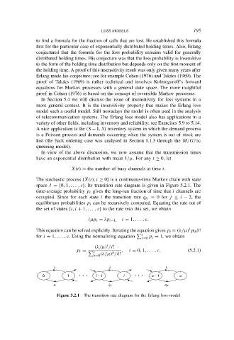
X(t) = the number of busy channels at time t.

The stochastic process {X(t), t ≥ 0} is a continuous-time Markov chain with state
space I = {0, 1, . . . , c}. Its transition rate diagram is given in Figure 5.2.1. The
time-average probability p i gives the long-run fraction of time that i channels are
occupied. Since for each state i the transition rate q ij = 0 for j ≤ i − 2, the
equilibrium probabilities p i can be recursively computed. Equating the rate out of
the set of states {i, i + 1, . . . , c} to the rate into this set, we obtain

iµp i = λp i−1, i = 1, . . . , c.
i
This equation can be solved explicitly. Iterating the equation gives p i = (λ/µ) p 0 /i!
c
for i = 1, . . . , c. Using the normalizing equation i=0 p i = 1, we obtain
i
(λ/µ) /i!
, i = 0, 1, . . . , c. (5.2.1)
p i = c k
k=0 (λ/µ) /k!
l l l
0 1 • • • i − 1 i • • • c − 1 c
m im cm

Figure 5.2.1 The transition rate diagram for the Erlang loss model