Page 325 - A First Course In Stochastic Models

320 ADVANCED RENEWAL THEORY

Analysis of the D-policy
For a given D-policy the stochastic process describing jointly the inventory of
unprocessed material and the status of the plant (on or off) is regenerative. The
epochs at which the plant is closed down are regeneration epochs. Define a cycle
as the time elapsed between two consecutive shutdowns. The long-run average cost
per time unit equals the value of E(cost incurred during one cycle) divided by the
value of E(expected length of one cycle). To find these two expected values, we
define the functions

α(x) = E(time until the buffer content exceeds the level D when the
current buffer content is D − x and there is no processing),
β(x) = E(holding costs incurred until the buffer content exceeds the level D
when the current buffer content is D − x and there is no processing)

for 0 ≤ x ≤ D. In particular, α(D) and β(D) denote the expected length of the
idle period in a cycle and the expected holding costs during that idle period. Also,
define the random variable γ D as the excess of the inventory over the level D

when the plant is reopened. Then E t(D + γ D ) and E h(D + γ D ) represent
the expected length of the busy period in a cycle and the expected holding cost
incurred during that busy period. Thus, under a given D-policy,

β(D) + K + E[h(D + γ D )]
the long-run average cost per time unit =
α(D) + E[t(D + γ D )]
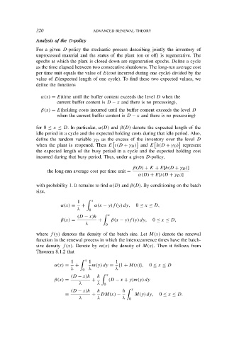
with probability 1. It remains to find α(D) and β(D). By conditioning on the batch
size,

1 x
α(x) = + α(x − y)f (y) dy, 0 ≤ x ≤ D,
λ 0
(D − x)h x
β(x) = + β(x − y)f (y) dy, 0 ≤ x ≤ D,
λ 0
where f (y) denotes the density of the batch size. Let M(x) denote the renewal
function in the renewal process in which the interoccurrence times have the batch-
size density f (x). Denote by m(x) the density of M(x). Then it follows from
Theorem 8.1.2 that

1 x 1 1
α(x) = + m(y) dy = {1 + M(x)}, 0 ≤ x ≤ D
λ 0 λ λ
(D − x)h h x
β(x) = + (D − x + y)m(y) dy
λ λ 0
(D − x)h h h x
= + DM(x) − M(y) dy, 0 ≤ x ≤ D.
λ λ λ 0