Page 330 - A First Course In Stochastic Models

ALTERNATING RENEWAL PROCESSES 325

(A.7) in Appendix A, we find
∞

E(τ down ) = P {R − L > t | R > L} dt
0
1 ∞ ∞
= {1 − G R (x + t)}f L (x) dx dt
q 0 0
1 ∞ ∞
= f L (x) {1 − G R (u)} du dx,
q 0 x
where the latter equality uses an interchange of the order of integration. Interchang-
ing again the order of integration, we next find that

1 ∞
E(τ down ) = {1 − G R (u)}F L (u) du.
q 0
We are now in a position to calculate an approximation for the probability dis-
tribution function of the total uptime in a time interval of given length t 0 when
the system has reached statistical equilibrium. An approximation to the desired
probability A(x, t 0 ) is obtained by applying formula (8.3.3) in which 1/α and 1/β
are replaced by E(τ up ) and E(τ down ) respectively. The numerical evaluation of the
right-hand side of (8.3.3) is easy, since the infinite series converges rapidly and
involves only Poisson probabilities. Numerical integration is required to calculate
the integrals for E(τ up ) and E(τ down ). It remains to investigate the quality of the
approximation for the probabilities A(x, t 0 ). Several assumptions have been made
to get the approximation. The most serious weakness of the approximation is the
assumption that the off-time is approximately exponentially distributed. Neverthe-
less it turns out that the approximation performs very well for practical purposes.
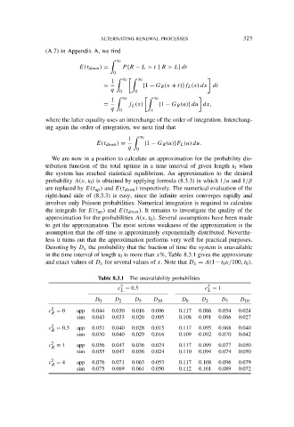
Denoting by D x the probability that the fraction of time the system is unavailable
in the time interval of length t 0 is more than x%, Table 8.3.1 gives the approximate
and exact values of D x for several values of x. Note that D x = A(1−t 0 x/100, t 0 ).

Table 8.3.1 The unavailability probabilities
2
2
c = 0.5 c = 1
L L
D 0 D 2 D 5 D 10 D 0 D 2 D 5 D 10
2
c = 0 app 0.044 0.030 0.016 0.006 0.117 0.086 0.054 0.024
R
sim 0.043 0.033 0.020 0.005 0.108 0.091 0.066 0.027
2
c = 0.5 app 0.051 0.040 0.028 0.015 0.117 0.095 0.068 0.040
R
sim 0.050 0.040 0.029 0.016 0.109 0.092 0.070 0.042
2
c = 1 app 0.056 0.047 0.036 0.024 0.117 0.099 0.077 0.050
R
sim 0.055 0.047 0.036 0.024 0.110 0.094 0.074 0.050
2
c = 4 app 0.076 0.071 0.063 0.053 0.117 0.108 0.096 0.079
R
sim 0.075 0.069 0.061 0.050 0.112 0.101 0.089 0.072