Page 326 - A First Course In Stochastic Models

ALTERNATING RENEWAL PROCESSES 321

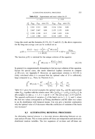
Table 8.2.1 Approximate and exact values for D
λ = 0.5 λ = 0.8
2
c D app D opt error (%) D app D opt error (%)
B
1
3 2.911 2.911 0.00 2.214 2.214 0.00
1 2.847 2.847 0.00 2.155 2.155 0.00
2
1 1 2.259 2.298 0.13 1.545 1.629 0.24
2
3 1.142 1.588 11.9 0.318 1.049 15.6

Using this result and the formulas (8.2.9), (8.1.7) and (8.1.2), the above expression
for the long-run average cost can be worked out as

D
Kλ(1 − λµ 1 ) − h D + M(y) dy
0 hλµ 2
g(D) = + hD + .
1 + M(D) 2(1 − λµ 1 )
The function g(D) is minimal for the unique solution of the equation
Kλ(1 − λµ 1 )
D
D + M(y) dy = . (8.2.10)
0 h
In general it is computationally demanding to find an exact solution of this equation.
Except for special cases, one needs numerical Laplace inversion to compute
x
0 M(y) dy; see Appendix F. However, an approximate solution to (8.2.10) is
easily calculated when it is assumed that the optimal value of D is sufficiently
large compared to µ 1 . Then, by Theorem 8.2.3,

D µ 2 µ 2 µ 3
D 2 2
M(y) dy ≈ + D 2 − 1 + 3 − 2 .
0 2µ 1 2µ 1 4µ 1 6µ 1
Table 8.2.1 gives for several examples the optimal value D opt and the approximate

value D app together with the relative error 100× g(D app ) − g(D opt )/g(D opt ) . In
all examples we take µ 1 = 1, h = 1 and K = 25. The arrival rate λ is 0.5 and 0.8.
2
1
1
1
The squared coefficient of variation c of the batch size is , , 1 and 3, where
B 3 2 2
the first two values correspond to an Erlang distribution and the latter two values
to an H 2 distribution with balanced means. Can you give a heuristic explanation
why the optimal value of D decreases when the coefficient of variation of the batch
size increases?
8.3 ALTERNATING RENEWAL PROCESSES
An alternating renewal process is a two-state process alternating between an on-
state and an off-state. The on-times and the off-times are independent and identically
distributed random variables. The two sequences of on-times and off-times are