Page 380 - A First Course In Stochastic Models

THE GI /G/1 QUEUE 375

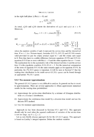
in the right half-plane {s|Re(s) > 0} and
′
′
a (0) − a (0)
2
1
α = .
a 2 (0)
As usual, a (0) and a (0) denote the derivatives of a 2 (s) and a 1 (s) at s = 0.
′
′
2 1
Moreover,
m−1

P delay = 1 − (1 − ρ)αa 2 (0) δ i (9.5.15)
i=1
and
m−1
′
′
ρ 2 2 a (0) a (0) 1
1
2
W q = E(S ) + E(A ) + 2E(S) − 2α + ,
2(1 − ρ)E(S) a 1 (0) a 2 (0) δ i
i=1
(9.5.16)
where the random variables S and A represent the service time and the interarrival
time. If m = 1 (i.e. Poisson input), formulas (9.5.13), (9.5.15) and (9.5.16) remain
valid provided we put the empty product equal to 1 and the empty sum equal
to 0. Note that there is a subtle difference between equations (9.5.9) and (9.5.14):
equation (9.5.9) has m roots with Re(s) > 0 and the other equation has m−1 roots.
The explanation lies in the asymmetric role of the interarrival time A and the service
time S in the ergodicity condition E(S)/E(A) < 1. For the numerical computation
of the roots of equation (9.5.14) the same remarks apply as for equation (9.5.9). In
particular, the P h/D/1 queue is important. It will be seen in Section 9.7 that the
waiting-time distribution in the multi-server GI/D/c queue can be found through
an appropriate P h/D/1 queue.
9.5.5 Two-moment Approximations
The general GI/G/1 queue is very difficult to analyse. In general one has to resort
to approximations. There are several approaches to obtain approximate numerical
results for the waiting-time probabilities:

(a) Approximate the service-time distribution by a mixture of Erlangian distribu-
tions or a Coxian-2 distribution.
(b) Approximate the continuous-time model by a discrete-time model and use the
discrete FFT method.

(c) Use two-moment approximations.

Approach (a) has been discussed in Sections 9.5.1 and 9.5.2. This approach
should only be used when the squared coefficient of variation of the service time
2
is not too large, say 0 ≤ c ≤ 2.
S
Let us now briefly discuss approach (b) for the GI/G/1 queue. This approach
is based on Lindley’s integral equation. Define the random variables