Page 440 - A First Course In Stochastic Models

A. USEFUL TOOLS IN APPLIED PROBABILITY 435

To see this, note that (A.7) implies

∞ ∞

k k 1/k
E(X ) = P {X > t} dt = P {X > t } dt
0 0
k
and next use the change of variable t = x .
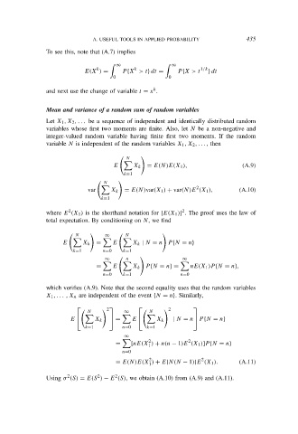
Mean and variance of a random sum of random variables

Let X 1 , X 2 , . . . be a sequence of independent and identically distributed random
variables whose first two moments are finite. Also, let N be a non-negative and
integer-valued random variable having finite first two moments. If the random
variable N is independent of the random variables X 1 , X 2 , . . . , then

N

E X k = E(N)E(X 1 ), (A.9)
k=1
N

2
var X k = E(N)var(X 1 ) + var(N)E (X 1 ), (A.10)
k=1
2
2
where E (X 1 ) is the shorthand notation for [E(X 1 )] . The proof uses the law of
total expectation. By conditioning on N, we find
N ∞ N

E X k = E X k | N = n P {N = n}
k=1 n=0 k=1

∞ n ∞

= E X k P {N = n} = nE(X 1 )P {N = n},
n=0 k=1 n=0
which verifies (A.9). Note that the second equality uses that the random variables
X 1 , . . . , X n are independent of the event {N = n}. Similarly,

2 2
   

N ∞ N

E  X k  = E  X k | N = n  P {N = n}
k=1 n=0 k=1
∞
2 2

= [nE(X ) + n(n − 1)E (X 1 )]P {N = n}
1
n=0
2
2
= E(N)E(X ) + E[N(N − 1)]E (X 1 ). (A.11)
1
2
2
2
Using σ (S) = E(S ) − E (S), we obtain (A.10) from (A.9) and (A.11).