Page 438 - A First Course In Stochastic Models

A. USEFUL TOOLS IN APPLIED PROBABILITY 433

Example A.2 The double-up strategy in roulette
In European roulette the wheel is divided in 37 sections, numbered as 1, . . . , 36
and 0. Of the sections numbered from 1 to 36, 18 are red and 18 are black. The
section marked 0 is assumed to be winning for the house. You have decided to bet
on 10 spins of the wheel and to use the double-up strategy. You bet each time on
red. Your initial bet is ¤1. You double your bet each time red does not come up.
If red appears, you start again with a bet of ¤1. You get paid twice your bet when
red comes up and you lose your bet otherwise. What is the expected value of your
loss after a playing round of 10 bets and what is the expected value of the total
amount you bet during the playing round?
To answer these questions, note that the betting process starts anew each time red
comes up except that fewer bets are left. Instead of considering 10 bets, consider
a playing round of n bets under the double-up strategy and define the random
variables L n and A n by

L n = the player’s loss after a playing round of n bets,
A n = the total amount the player bets in a playing round of n bets.

To compute the expected values of L n and A n , it is natural to condition on the
random variable Y denoting the number of spins of the wheel until red comes up
18
for the first time. Obviously, Y is geometrically distributed with parameter p = .
37
By conditioning on Y and noting that the player’s profit is ¤1 each time red comes
up, it follows that

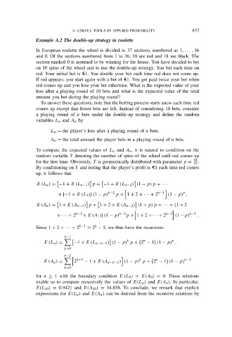
E (L n ) = −1 + E (L n−1 ) p + −1 + E (L n−2 ) (1 − p) p + · · ·

n
+ [−1 + E (L 1 )] (1 − p) n−2 p + 1 + 2 + · · · + 2 n−1 (1 − p) ,

E (A n ) = 1 + E (A n−1 ) p + 1 + 2 + E (A n−2 ) (1 − p) p + · · · + [1 + 2

+ · · · + 2 n−2 + E (A 1 )] (1 − p) n−2 p + 1 + 2 +· · ·+ 2 n−1 (1 −p) n−1 .
k
Since 1 + 2 + · · · + 2 k−1 = 2 − 1, we thus have the recursions
n−1

k n n
E (L n ) = −1 + E (L n−k−1 ) (1 − p) p + 2 − 1 (1 − p) ,
k=0

n−2
k+1 k n n−1
E (A n ) = 2 − 1 + E (A n−k−1 ) (1 − p) p + 2 − 1 (1 − p)
k=0
for n ≥ 1 with the boundary condition E (L 0 ) = E(A 0 ) = 0. These relations
enable us to compute recursively the values of E(L n ) and E(A n ). In particular,
E(L 10 ) = 0.9421 and E(A 10 ) = 34.858. To conclude, we remark that explicit
expressions for E(L n ) and E(A n ) can be derived from the recursive relations by