Page 437 - A First Course In Stochastic Models

432 APPENDICES

when Y has a continuous distribution with probability density f (y). The law of
total expectation and the law of total probability will be frequently used in this
book. We illustrate these laws by two examples.

Example A.1 Service with interruptions
A single unloader is available to unload ships. The unloading time U of a ship
has a given probability density f (t) with finite mean γ . The unloading process,
however, is subject to interruptions. Those interruptions have exogenous causes and
occur according to a Poisson process with rate λ. The durations of the interruptions
are independent and identically distributed random variables with mean δ. After
an interruption the unloading of the ship is resumed at the point it was stopped
by the interruption. What is the expected amount of time needed to complete the
unloading of the ship?
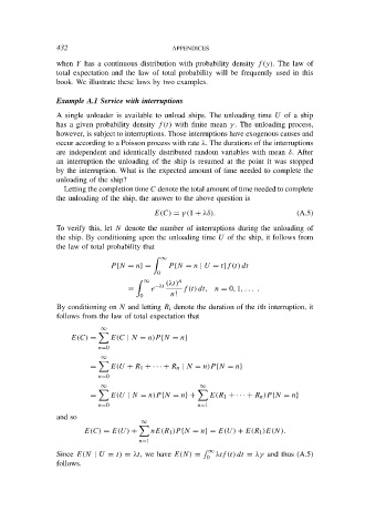
Letting the completion time C denote the total amount of time needed to complete
the unloading of the ship, the answer to the above question is
E(C) = γ (1 + λδ). (A.5)
To verify this, let N denote the number of interruptions during the unloading of
the ship. By conditioning upon the unloading time U of the ship, it follows from
the law of total probability that
∞

P {N = n} = P {N = n | U = t}f (t) dt
0
∞ (λt)
n
−λt
= e f (t) dt, n = 0, 1, . . . .
0 n!
By conditioning on N and letting R i denote the duration of the ith interruption, it
follows from the law of total expectation that
∞

E(C) = E(C | N = n)P {N = n}
n=0
∞

= E(U + R 1 + · · · + R n | N = n)P {N = n}
n=0
∞ ∞

= E(U | N = n)P {N = n} + E(R 1 + · · · + R n )P {N = n}
n=0 n=1
and so
∞

E(C) = E(U) + nE(R 1 )P {N = n} = E(U) + E(R 1 )E(N).
n=1

∞
Since E(N | U = t) = λt, we have E(N) = λtf (t) dt = λγ and thus (A.5)
0
follows.