Page 77 - A First Course In Stochastic Models

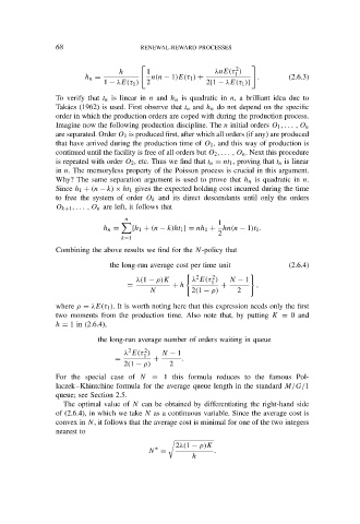
68 RENEWAL-REWARD PROCESSES

2
h 1 λnE(τ )
1
h n = n(n − 1)E(τ 1 ) + . (2.6.3)
1 − λE(τ 1 ) 2 2{1 − λE(τ 1 )}
To verify that t n is linear in n and h n is quadratic in n, a brilliant idea due to
Tak´ acs (1962) is used. First observe that t n and h n do not depend on the specific
order in which the production orders are coped with during the production process.
Imagine now the following production discipline. The n initial orders O 1 , . . . , O n
are separated. Order O 1 is produced first, after which all orders (if any) are produced
that have arrived during the production time of O 1 , and this way of production is
continued until the facility is free of all orders but O 2 , . . . , O n . Next this procedure
is repeated with order O 2 , etc. Thus we find that t n = nt 1 , proving that t n is linear
in n. The memoryless property of the Poisson process is crucial in this argument.
Why? The same separation argument is used to prove that h n is quadratic in n.
Since h 1 + (n − k) × ht 1 gives the expected holding cost incurred during the time
to free the system of order O k and its direct descendants until only the orders
O k+1 , . . . , O n are left, it follows that
n
1

h n = {h 1 + (n − k)ht 1 } = nh 1 + hn(n − 1)t 1 .
2
k=1
Combining the above results we find for the N-policy that
the long-run average cost per time unit (2.6.4)

2 2
λ(1 − ρ)K λ E(τ ) N − 1
1
= + h + ,
N 2(1 − ρ) 2
where ρ = λE(τ 1 ). It is worth noting here that this expression needs only the first
two moments from the production time. Also note that, by putting K = 0 and
h = 1 in (2.6.4),
the long-run average number of orders waiting in queue
2
2
λ E(τ ) N − 1
1
= + .
2(1 − ρ) 2
For the special case of N = 1 this formula reduces to the famous Pol-
laczek–Khintchine formula for the average queue length in the standard M/G/1
queue; see Section 2.5.
The optimal value of N can be obtained by differentiating the right-hand side
of (2.6.4), in which we take N as a continuous variable. Since the average cost is
convex in N, it follows that the average cost is minimal for one of the two integers
nearest to

2λ(1 − ρ)K
∗
N = .
h