Page 140 - A Practical Companion to Reservoir Stimulation

STIMULATION OF HORIZONTAL WELLS

EXAMPLE 5-2
graphs are plotted for skins equal to 0 and 2, which indicate
Material Balance Calculation for a very moderate damage. After a year (from the emergence of
Reservoir with a Horizontal Well boundaries), the cumulative production will be 8 x 10' SCF
for s = 0 and 5.5 x lo8 SCF for s = 2. This is a substantial
Suppose that a 500-ft horizontal well is drilled in a reservoir difference, again indicating the need for careful stimulation.
with the variables shown in Table 5-2. Forecast the perfor-
mance for a closed reservoir configuration.

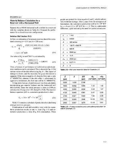
Solution (Ref. Section 19-2) k = 1md
At first, an estimation of minimum reserves should be calcu- yo ,= 0.633
lated assuming h = 15 ft and A = 320 acres: I
I A . = 320acres
Ah@S, (320) (43,560) (15) (0.1) (0.6) I T = 190"F=65OoR I
G. = ~ -
-
Bh' (0.00347) I
I L = 500ft
-
= 3.6 x lo9 SCF. p = 5300psi
The value of B, in resft3/SCF is calculated by h = 15ft
I pwr = 2500psi I
I r, = 0.271 ft I

Then, a forecast of performance at stabilized pseudosteady- I P = 3
state conditions can be calculated. This is shown in Fig. J-2 for Table J-2-Well and reservoir data for Example J-2.
various values of the skin effect using Eq. J- 1. The impact of
damage is shown, and the necessity for good stimulation is
apparent. If the skin is equal to +5, then the flow rate is only
1.7 MMSCF/d; whereas if the skin effect is eliminated by
aggressive stimulation, the flow rate will be 4.3 MMSCF/d.
A long-term forecast of performance was then calculated,
incorporating gas material balance and the horizontal well
deliverability. Since the initial pressure is taken as 5300 psi
and since the Zis equal to 1.03, thenp/Z= 5 146. The material
balance equation (P/Z vs. cumulative production) is then
iz)
G,, = 3.6 x 109-7 x lo5 . (5-6)

Table 5-3 contains a schedule of production for a declining
average reservoir pressure.
Combination of well deliverability (rate) with the cumu- Table J-3- Pressure decline and cumulative production for
lative production results in rate vs. time (Fig. 5-3) and cu- well in Example J-2.
mulative production vs. time (Fig. 5-4) relationships. These

5-3