Page 355 - Acquisition and Processing of Marine Seismic Data

346 6. DECONVOLUTION

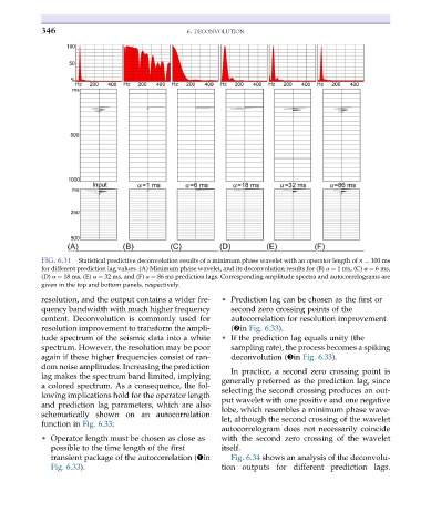
FIG. 6.31 Statistical predictive deconvolution results of a minimum phase wavelet with an operator length of n ¼ 100 ms
for different prediction lag values. (A) Minimum phase wavelet, and its deconvolution results for (B) α ¼ 1 ms, (C) α ¼ 6ms,
(D) α ¼ 18 ms, (E) α ¼ 32 ms, and (F) α ¼ 86 ms prediction lags. Corresponding amplitude spectra and autocorrelograms are
given in the top and bottom panels, respectively.
resolution, and the output contains a wider fre- • Prediction lag can be chosen as the first or
quency bandwidth with much higher frequency second zero crossing points of the
content. Deconvolution is commonly used for autocorrelation for resolution improvement
resolution improvement to transform the ampli- (➋in Fig. 6.33).
tude spectrum of the seismic data into a white • If the prediction lag equals unity (the
spectrum. However, the resolution may be poor sampling rate), the process becomes a spiking
again if these higher frequencies consist of ran- deconvolution (➌in Fig. 6.33).
dom noise amplitudes. Increasing the prediction
In practice, a second zero crossing point is
lag makes the spectrum band limited, implying
generally preferred as the prediction lag, since
a colored spectrum. As a consequence, the fol-
selecting the second crossing produces an out-
lowing implications hold for the operator length
put wavelet with one positive and one negative
and prediction lag parameters, which are also
lobe, which resembles a minimum phase wave-
schematically shown on an autocorrelation
let, although the second crossing of the wavelet
function in Fig. 6.33:
autocorrelogram does not necessarily coincide
• Operator length must be chosen as close as with the second zero crossing of the wavelet
possible to the time length of the first itself.
transient package of the autocorrelation (➊in Fig. 6.34 shows an analysis of the deconvolu-
Fig. 6.33). tion outputs for different prediction lags.