Page 439 - Acquisition and Processing of Marine Seismic Data

430 9. VELOCITY ANALYSIS

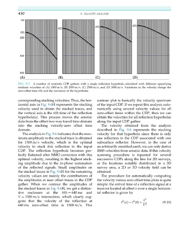
FIG. 9.5 A number of synthetic CDP gathers with a single reflection hyperbola calculated with different upperlying
medium velocities of (A) 1400 m/s, (B) 2000 m/s, (C) 2500 m/s, and (D) 3000 m/s. Variations in the velocity change the
zero-offset time t(0) and the curvature of the hyperbolas.

corresponding stacking velocities. Thus, the hor- contour plot is basically the velocity spectrum
izontal axis in Fig. 9.6H represents the stacking of the input CDP. If we repeat this analysis auto-
velocity used to obtain the stacked traces, and matically using several velocity values for all
the vertical axis is the t(0) time of the reflection zero-offset times within the CDP, then we can
hyperbola(s). This process moves the seismic obtain the velocities for all reflection hyperbolas
data from the offset two-way travel time domain along the input CDP gather.
into the stacking velocity-zero offset time The velocity obtained from the analysis
domain. described in Fig. 9.6 represents the stacking
The analysis in Fig. 9.6 indicates that the max- velocity for that hyperbola since there is only
imum amplitude in the stacked trace is obtained one reflection in the CDP associated with one
for 1500 m/s velocity, which is the optimal subsurface reflector. However, in the case of
velocity to stack this reflection in the input an arbitrarily stratified earth, we can only derive
CDP. The reflection hyperbola becomes per- RMS velocities from seismic data. If this velocity
fectly flattened after NMO correction with this scanning procedure is repeated for several
optimal velocity, resulting in the highest stack- successive CDPs along the line for 2D surveys,
ing amplitude due to the in-phase summation or the locations suitably distributed in a 3D
of the reflected signals. Small amplitudes on survey area, a 2D or 3D velocity field can be
the stacked traces in Fig. 9.6H for the remaining obtained.
velocity values are mainly the contributions of The procedure for automatically computing
the amplitudes at near offset traces in the CDP the velocity versus zero offset time plots is quite
gather. When we contour the amplitudes of simple: the arrival time of a reflection signal at a
the stacked traces in Fig. 9.6H, we get a distinc- receiver located at offset x over a single horizon-
tive enclosure at the t(0) ¼ 640 ms and tal reflector is given by
V ¼ 1500 m/s intersection, which clearly sug- 2
gests that the velocity of the reflection at t xðÞ ¼ t 0ðÞ + x (9.10)
2
2
640 ms zero-offset time is 1500 m/s. This V 2