Page 104 - Adaptive Identification and Control of Uncertain Systems with Nonsmooth Dynamics

Adaptive Control for Manipulation Systems 97

2) An exponential component h 2 (v) is utilized to denote the Stribeck ef-
fect, where the convergence rate is related to the critical velocity.
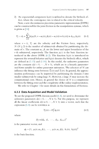
Now, a new discontinuous piecewise parametric representation (DPPR)
can be constructed for the joint friction in the manipulation systems, which
is given as [14]

N

T f = d 0 + [d r ρ r (0,v − α r (v),β r (v) − α r (v)) + h 1 (v)]+ d N+1h 2 (v) (6.4)
r=1
where v =˙x, T f are the velocity and the friction force, respectively.
N (N ≥ 2) is the number of subintervals obtained by partitioning the do-
main of v. The constants α r , β r are the lower and upper boundaries of the
r-th subinterval, respectively. The function ρ r (·) is the basic function in-
troduced in the above DPPR (6.2). The function h 1 (v) is introduced to
represent the reversal behavior and h 2 (v) denotes the Stribeck effect, which
are defined in (1.15)and (1.16). In this model, the unknown parameters
are the constants d i (i = 0,··· ,N + 1), which are in a linearly parameter-
ized form suitable for online parameter estimation. The selection of N can
ˆ
influence the fitting error between T f (v) and T f (v). In general, the approx-
imation performance can be improved by partitioning the domain I into
smaller subintervals by using large N.However,alarge N may increase the
computational costs. Hence, in general the choice of N is a compromise
between the fitting error and the complexity of the online implementation.
We refer to Chapter 1 for more details on this formulation of frictions.

6.3.3 Data Acquisition and Model Validation

To use the proposed DPPR friction model (6.4), we need to determine the
unknown parameters d i (i = 0,··· ,N + 1). For this purpose, we represent
all the linear coefficients d i (i = 0,··· ,N + 1) into a vector, such that the
expression (6.4) can be rewritten as
T
T f (v) = D φ f (v) (6.5)
f
where
T
D f =[d 0 , d 1 , ··· , d N , d N+1 ]
is the parameter vector, and

T
φ f =[1,ρ 1 (v,α 1 ,β 1 ), ··· ,ρ r (v,α r ,β r ), h 1 (v), h 2 (v)]
is the basis function.