Page 108 - Adaptive Identification and Control of Uncertain Systems with Nonsmooth Dynamics

Adaptive Control for Manipulation Systems 101

The adaptive law for online updating D is given by

T
˙ D =−
γ(χ)e − σ
e v D (6.12)
v
where
> 0 is the learning gain matrix, σ> 0 is a scalar used in the
e-modification scheme to guarantee the boundedness of D.
Substituting (6.10)and (6.11)into(6.9), one can have the closed-loop
error dynamics as

T
M(x)˙e v =−K pe v − ˜ D φ(χ) − C(x, ˙x)e v −
(6.13)
∗
where ˜ D = D − D is the parameter estimation error.
Now, the main results of this chapter can be summarized as follows:

Theorem 6.1. Consider the manipulation system described by (6.1) with friction
dynamics given in (6.5). The control (6.11) is implemented by incorporating the
DPPR friction model (6.4) into the augmented DPPR (6.10), and using the
adaptive law (6.12), then the tracking errors e v ,e and the parameter estimation error
˜ D are all uniformly ultimately bounded, and will converge to small compact sets
around zero, which are defined in (6.19), (6.20), and (6.22), respectively.

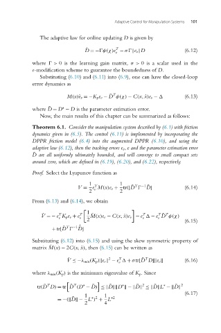
Proof. Select the Lyapunov function as
1 1
−1
T
T
˜
V = e M(x)e v + tr([ ˜ D
D] (6.14)
v
2 2
From (6.13)and (6.14), we obtain
1

T
T
T
T
˙ V =− e K pe v + e T ˙ M(x)e v − C(x, ˙x)e v − e
− e ˜ D φ(χ)
v v v v
2 (6.15)
T −1 ˙
˜
+ tr[ ˜ D
D]
Substituting (6.12)into(6.15) and using the skew symmetric property of
matrix ˙ M(x) − 2C(x, ˙x),then(6.15) can be written as
2 T T
˙ V ≤−λ min (K p ) e v − e
+ σtr[ ˜ D D] e v (6.16)
v
where λ min (K p ) is the minimum eigenvalue of K p. Since

T T 2 2
∗
∗
∗
tr( ˜ D D) = tr ˜ D (D − ˜ D) ≤ ˜ D D − ˜ D ≤ ˜ D L − ˜ D
(6.17)
1 ∗ 2 1 ∗2
=−( ˜ D − L ) + L
2 4