Page 105 - Adaptive Identification and Control of Uncertain Systems with Nonsmooth Dynamics

98 Adaptive Identification and Control of Uncertain Systems with Non-smooth Dynamics

It should be mentioned that D f can be estimated offline by using the
collected data and the recursive least squares (LS) estimator. Specifically, it
is noted that the instantaneous friction effect such as the Stribeck effect
vanishes when the motion velocity is a constant, such that the dynam-
ics (6.1)become T f ≈ τ for constant velocities. As a consequence, T f can
be practically obtained by measuring the motor torque, and thus used for
the model identification. For instance, in our studies, the used experiment
platform is a 3-link manipulator system, which is equipped with three
permanent-magnet alternating current servomotors configured with ab-
solute incremental encoders. Hence, the actual joint rotation angles are
measured using these encoders and the joint motions are controlled by a
motion control implemented in DSP56303 Turbo PMAC made by Mo-
torola.
The experimental data acquisition process is as follows. Firstly, we deter-
mine the forward velocity range [0,v max ] and reverse velocity range [v min ,0]
under the working condition of the system. Then, two groups of friction
torque data can be obtained respectively within [0,v max ] and [v min ,0],thatis,
{(v p1 ,F p1 ),··· ,(v pl ,F pl )} in the forward range and {(v n1 ,F n1 ),··· ,(v nl ,F nl )}
in the reverse range, where l represents the total number of collected data.
Since the smallest torque is the Coulomb friction torque [1], we can find
from these two groups of data the Coulomb friction and its corresponding
velocity (v pc ,F pc ) and (v nc ,F nc ),where v pc and v nc are the Coulomb frictions
within forward and reverse motions, respectively. Moreover, in order to get
a better data set, we can repeat the experiment several times and then use
the average of the collected data for the modeling and controller designs.
Here, in this chapter, in order to show the validity of the proposed
DPPR friction model, we provide some simulations, which clearly illustrate
the approximation capabilities of the proposed parametric representation of
friction. Both the effectiveness of h 1 and h 2 are shown in these examples.
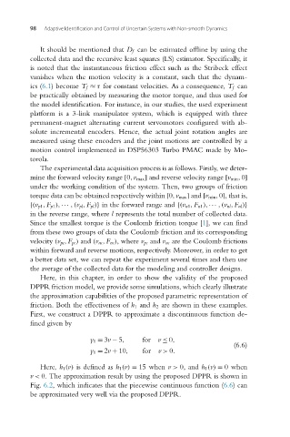
First, we construct a DPPR to approximate a discontinuous function de-
fined given by

y 1 = 3v − 5, for v ≤ 0,
(6.6)
y 1 = 2v + 10, for v > 0.

Here, h 1 (v) is defined as h 1 (v) = 15 when v > 0, and h 1 (v) = 0when
v < 0. The approximation result by using the proposed DPPR is shown in
Fig. 6.2, which indicates that the piecewise continuous function (6.6)can
be approximated very well via the proposed DPPR.