Page 110 - Adaptive Identification and Control of Uncertain Systems with Nonsmooth Dynamics

Adaptive Control for Manipulation Systems 103

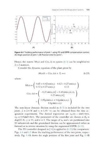
Figure 6.4 Tracking performance of joint 1 using PD and DPPR compensation control.
(A) Angle position of joint 1; (B) Position error for joint 1.

Hence, the matrix M(x) and C(x, ˙x) in system (6.1) can be simplified to
2 × 2 matrices.
Consider the dynamic equation of the plant given by

M(x)¨x + C(x, ˙x)˙x + T f = τ (6.23)

where

0.65 + 0.42cos(x 2 ) 0.12 + 0.27cos(x 2 )
M(x) =
0.12 + 0.27cos(x 2 ) 0.12

2
−0.21sin(x 2 )˙x − 0.42sin(x 2 )˙x 1 ˙x 2
2
C(x, ˙x)˙x = 2
0.21sin(x 2 )˙x
2

1.85g sin(x 1 ) + 0.6g sin(x 1x 2 )
+
0.6g sin(x 1x 2 )
The non-linear dynamic friction model in (6.7) is included for the two
joints. f s = 2.4 N and v c = 1.05 /s can be obtained from the data ac-
◦
quisition experiments. The desired trajectories are x d1 (t) = sin(0.4πt),
x d2 = 0.8sin(0.4πt). The parameters of the controller are chosen as K p =
diag(22,8), γ = 10, and σ = 3. The ranges of x d and e are partitioned into
50 subintervals and the generalized friction can be approximated either in
forward or in reverse situation by using the augmented DPPR (6.10).
The PD controller designed in [16]isappliedto(6.23) for comparison.
Figs. 6.4 and 6.5 show the tracking performance of the two joints, respec-
tively. Fig. 6.4A shows the angle position of the first joint and Fig. 6.4B