Page 124 - Adaptive Identification and Control of Uncertain Systems with Nonsmooth Dynamics

120 Adaptive Identification and Control of Uncertain Systems with Non-smooth Dynamics

was also handled together with other system uncertainties by using NNs in
[12,15], where the dead-zone dynamics are reformulated in (7.9). However,
in these NN-based control designs, only uniform ultimate boundedness of
the control error can be guaranteed.
In this chapter, an adaptive robust finite-time neural-network control
(ARFTNC) is designed for PMSM servo systems with model uncertainties
and unknown non-linear dead-zone input [28]. An alternative fast termi-
nal sliding mode control (FTSMC) is developed by modifying the sliding
manifold, where the singularity problem in the conventional TSMC ap-
proaches is avoided. Moreover, an NN is used to handle the unknown
system uncertainties and the induced dynamics by dead-zone. It is proved
that finite-time stability in both the reaching phase and the sliding phase
can be guaranteed. Comparative experiments are conducted to validate the
effectiveness and superior performance of the proposed method.

8.2 PROBLEM FORMULATION AND PRELIMINARIES
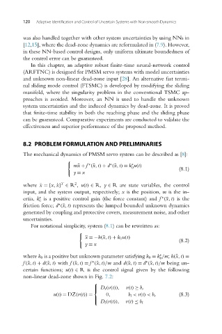
The mechanical dynamics of PMSM servo system can be described as [8]:

∗
∗
∗
m¨x + f (¯x,t) + d (¯x,t) = k u(t)
0 (8.1)
y = x
T
2
where ¯x =[x, ˙x] ∈ R , u(t) ∈ R, y ∈ R are state variables, the control
input, and the system output, respectively; x is the position, m is the in-
ertia, k is a positive control gain (the force constant) and f (¯x,t) is the
∗
∗
0
friction force; d (¯x,t) represents the lumped bounded unknown dynamics
∗
generated by coupling and protective covers, measurement noise, and other
uncertainties.
For notational simplicity, system (8.1) can be rewritten as:

¨ x =−h(¯x,t) + k 0u(t)
(8.2)
y = x
∗
where k 0 is a positive but unknown parameter satisfying k 0 = k /m; h(¯x,t) =
0
∗
∗
f (¯x,t) + d(¯x,t) with f (¯x,t) = f (¯x,t)/m and d(¯x,t) = d (¯x,t)/m being un-
certain functions; u(t) ∈ R is the control signal given by the following
non-linear dead-zone shown in Fig. 7.2:
⎧
⎪ D r (v(t)), v(t) ≥ b r
⎨
u(t) = DZ(v(t)) = 0, b l < v(t)< b r (8.3)
⎪
D l (v(t)), v(t) ≤ b l
⎩