Page 181 - Adaptive Identification and Control of Uncertain Systems with Nonsmooth Dynamics

178 Adaptive Identification and Control of Uncertain Systems with Non-smooth Dynamics

form, where the state feedback control of the original system is transformed
into an output feedback control problem of the transformed system. A sim-
ilar idea was also reported in [9] for pure-feedback control systems.
In this chapter, a modified output feedback control is investigated for a
class of non-linear pure-feedback systems with unknown input dead-zone.
First, new system states and the coordinate transform are introduced such
that the considered non-linear pure-feedback system can be transformed
into the Brunovsky form [10], which is particularly suitable for control de-
signs. With this idea, the problem is reformulated as the output feedback
control of the derived canonical system, where the lumped uncertainties
caused by the unknown dead-zone and other uncertainties are defined as
an extended state and compensated by employing an ESO. Tracking differ-
entiator (TD) is also used in the adaptive dynamic surface control (DSC)
design procedure to enhance convergence speed. Moreover, similar to the
previous chapters, the dead-zone is represented as a linear system with a
linear time-varying gain and a bounded disturbance. The stability analysis
is provided based on the Lyapunov synthesis, and simulation results validate
the effectiveness of the proposed method.

11.2 PROBLEM FORMULATION AND PRELIMINARIES
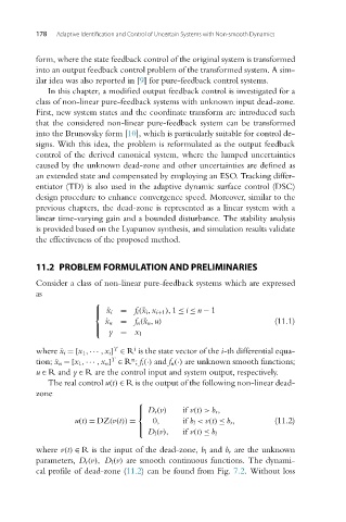
Consider a class of non-linear pure-feedback systems which are expressed
as
⎧
= f i (¯x i ,x i+1 ),1 ≤ i ≤ n − 1
⎪ ˙ x i
⎨
˙ x n = f n (¯x n ,u) (11.1)
⎪
⎩
y = x 1
T
i
where ¯x i =[x 1 ,··· ,x i ] ∈ R is the state vector of the i-thdifferentialequa-
n
T
tion; ¯x n =[x 1 ,··· ,x n ] ∈ R ; f i (·) and f n (·) are unknown smooth functions;
u ∈ Rand y ∈ R are the control input and system output, respectively.
The real control u(t) ∈ R is the output of the following non-linear dead-
zone
⎧
⎪ D r (v) if v(t)> b r ,
⎨
u(t) = DZ(v(t)) = 0, if b l < v(t) ≤ b r , (11.2)
⎪
D l (v), if v(t) ≤ b l
⎩
where v(t) ∈ R is the input of the dead-zone, b l and b r are the unknown
parameters, D r (v), D l (v) are smooth continuous functions. The dynami-
cal profile of dead-zone (11.2) can be found from Fig. 7.2. Without loss