Page 47 - Adaptive Identification and Control of Uncertain Systems with Nonsmooth Dynamics

38 Adaptive Identification and Control of Uncertain Systems with Non-smooth Dynamics

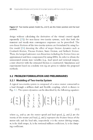
Figure 3.1 Two-inertia system model (θ m and θ are the motor position and the load
l
position).

design without calculating the derivatives of the virtual control signals
repeatedly [25]) for non-linear two-inertia systems, such that both the
transient and steady-state convergence responses can be prescribed. The
non-linear frictions of the two-inertia systems are formulated by using Lu-
Gre model [26] denoting the effect of major friction dynamics such as
Coulomb friction, Viscous friction, Static friction, and Stribeck friction.
Then, the lumped unknown non-linearities including the friction force are
approximated and then compensated by using ESNs. In order to obtain the
unmeasured system state variables (e.g., load speed and torsional torque),
a state observer with the estimated friction is constructed. Simulations and
experiments based on a realistic test-rig are given to validate the proposed
methods.

3.2 PROBLEM FORMULATION AND PRELIMINARIES

3.2.1 Modeling of Two-Inertia System
A typical two-inertia system is composed of a servo motor connected to
a load through a stiffness shaft and flexible coupling, which is shown in
Fig. 3.1. The system dynamics can be described by the following equation:

⎛ ⎞
−b f 1 b f
⎛ ⎞ ⎛ ⎞ ⎛ ⎞ ⎛ f l ⎞
0
ω l ⎜ J l J l J l ⎟ ω l J l
⎜ ⎟
⎟ ⎜ ⎟ ⎜ ⎟ ⎜ ⎟
d ⎜
⎝ m s ⎠ = ⎜ −k f 0 k f ⎟
dt ⎜ ⎟ ⎝ m s ⎠ + ⎝ 0 ⎠ u − ⎝ 0 ⎠
1
⎝ b f 1 ⎠ f m
ω m −b f ω m
J m J m
J m J m J m
(3.1)
where ω m and ω l are the motor speed and load speed, J m and J l are the
inertia of the motor and load, f m and f l represent the friction forces of the
motor side and the load side, respectively. u is the motor driving torque,
m s is the shaft torque, k f is the torsional stiffness coefficient, b f is the damp-
ing coefficient.