Page 49 - Adaptive Identification and Control of Uncertain Systems with Nonsmooth Dynamics

40 Adaptive Identification and Control of Uncertain Systems with Non-smooth Dynamics

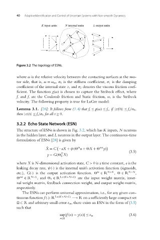
Figure 3.2 The topology of ESNs.

where ω is the relative velocity between the contacting surfaces at the mo-
tor side, that is, ω = ω m, σ 0 is the stiffness coefficient, σ 1 is the damping
coefficient of the internal state z,and σ 2 denotes the viscous friction coef-
ficient. The function g(ω) is chosen to capture the Stribeck effect, where
f c and f s are the Coulomb friction and Static friction, ω s is the Stribeck
velocity. The following property is true for LuGre model:
Lemma 3.1. [26]: It follows from (3.4)that f c ≤ g(ω) ≤ f s,if |z(0)|≤ f s /σ 0,
then |z(t)|≤ f s /σ 0 for all t ≥ 0.

3.2.2 Echo State Network (ESN)
The structure of ESNs is shown in Fig. 3.2, which has K inputs, N neurons
in the hidden layer, and L neurons in the output layer. The continuous-time
formulation of ESNs [28]isgiven by

in out
˙ X = C −aX + ψ( u + X + y)
(3.5)
T
y = G( X)
0
where X is N-dimensional activation state, C > 0 is a time constant, a is the
leaking decay rate, ψ(·) is the internal unit’s activation function (sigmoids,
in
etc.), G(·) is the output activation function. ∈ R N×K , ∈ R N×N ,
out ∈ R N×L ,and 0 ∈ R L×(K+N+L) are the input weight matrix, inter-
nal weight matrix, feedback connection weight, and output weight matrix,
respectively.
The ESNs can perform universal approximation, i.e., for any given con-
tinuous function f (·):R L×(K+N+L) −Ð R on a sufficiently large compact set
⊂ R and arbitrary small error ε m, there exists an ESN in the form of (3.5)
such that

sup|f (x) − y(x)|≤ ε m (3.6)
x∈