Page 71 - Adaptive Identification and Control of Uncertain Systems with Nonsmooth Dynamics

62 Adaptive Identification and Control of Uncertain Systems with Non-smooth Dynamics

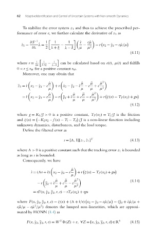
To stabilize the error system z 1 and thus to achieve the prescribed per-
formance of error e, we further calculate the derivative of z 1 as
∂S −1 1 1 1
˙ e e ˙μ
˙
˙ z 1 = λ = − − = r x 2 −¨y d − e ˙μ/μ
∂λ 2 λ + δ λ − δ ¯ μ μ 2
(4.11)

1 1 1
where r = − can be calculated based on e(t), μ(t) and fulfills
2μ λ+δ λ− ¯ δ
0 < r ≤ r M for a positive constant r M .
Moreover, one may obtain that
2
˙ μ ˙ μ ¨ μ ˙ μ
¨ z 1 =˙ x 2 −¨y d − e + r ˙ x 2 −¨y d −¨e − e + e
r
μ μ μ μ 2
2
˙ μ ˙ μ ¨ μ ˙ μ
=˙ r x 2 −¨y d − e − r ¨ y d +˙e + e − e + r ζ(x) − T F (x 2 ) + gu
μ μ μ μ 2
(4.12)
where g = K 1 /J > 0 is a positive constant, T F (x 2 ) = T f /J is the friction

and ζ(x) = −K 2x 2 − f (x) − T l − T d /J is a non-linear function including
unknown dynamics, disturbances, and the load torque.
Define the filtered error as
T
s =[
,1][z 1 , ˙z 1 ] (4.13)

where
> 0 is a positive constant such that the tracking error z 1 is bounded
as long as s is bounded.
Consequently, we have

˙ μ
r
s ˙ = (
r +˙) x 2 −¨y d − e + r ζ(x) − T F (x 2 ) + gu
μ
2
˙ μ ¨ μ ˙ μ (4.14)
− r ¨ y d +˙e + e − e
μ μ μ 2
= rF(x, ˙y d , ¨y d ,r,e) − rT F (x 2 ) + rgu

where F(x, ˙y d , ¨y d ,r,e) = ζ(x) + (
+˙r/r) x 2 −¨y d − e ˙μ/μ − (¨y d +˙e ˙μ/μ +
2
2
e ¨μ/μ − e ˙μ /μ ) denotes the lumped non-linearities, which are approxi-
mated by HONN (4.4)as
T
F(x, ˙y d , ¨y d ,r,e) = W (Z) + ε, ∀Z =[x, ˙y d , ¨y d ,r,e]∈ R 6 (4.15)