Page 25 - Advanced_Engineering_Mathematics o'neil

1.1 Terminology and Separable Equations 5

2

1.5

1

0.5

0
x
–0.6 –0.4 –0.2 0 0.2 0.4 0.6
–0.5

–1

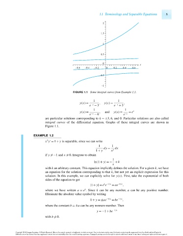
FIGURE 1.1 Some integral curves from Example 1.1.

1 1
y(x) = , y(x) = ,
e −x − 3 e −x + 3
1 1
y(x) = , and y(x) = = e x
e −x − 6 e −x
are particular solutions corresponding to k =±3,6, and 0. Particular solutions are also called
integral curves of the differential equation. Graphs of these integral curves are shown in
Figure 1.1.

EXAMPLE 1.2
2
x y = 1 + y is separable, since we can write

1 1
dy = dx
1 + y x 2
if y =−1 and x = 0. Integrate to obtain
1
ln|1 + y|=− + k
x
with k an arbitrary constant. This equation implicitly defines the solution. For a given k,wehave
an equation for the solution corresponding to that k, but not yet an explicit expression for this
solution. In this example, we can explicitly solve for y(x). First, take the exponential of both
sides of the equation to get
k −1/x
|1 + y|= e e = ae −1/x ,
k
where we have written a = e . Since k can be any number, a can be any positive number.
Eliminate the absolute value symbol by writing
1 + y =±ae −1/x = be −1/x ,
where the constant b =±a can be any nonzero number. Then

y =−1 + be −1/x
with b = 0.

Copyright 2010 Cengage Learning. All Rights Reserved. May not be copied, scanned, or duplicated, in whole or in part. Due to electronic rights, some third party content may be suppressed from the eBook and/or eChapter(s).
Editorial review has deemed that any suppressed content does not materially affect the overall learning experience. Cengage Learning reserves the right to remove additional content at any time if subsequent rights restrictions require it.

October 14, 2010 14:9 THM/NEIL Page-5 27410_01_ch01_p01-42