Page 576 - Advanced_Engineering_Mathematics o'neil

556 CHAPTER 15 Special Functions and Eigenfunction Expansions

0.2

0.1
0
–0.2 0 0.2 0.4 0.6 0.8 1 1.2
x
–0.1

–0.2

–0.3

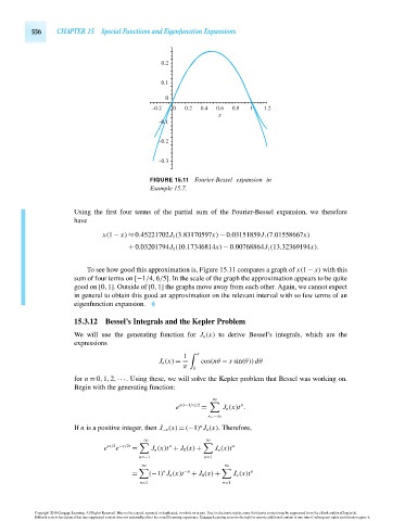
FIGURE 15.11 Fourier-Bessel expansion in
Example 15.7.

Using the first four terms of the partial sum of the Fourier-Bessel expansion, we therefore
have
x(1 − x) ≈ 0.45221702J 1 (3.83170597x) − 0.03151859J 1 (7.01558667x)
+ 0.03201794J 1 (10.17346814x) − 0.00768864J 1 (13.32369194x).

To see how good this approximation is, Figure 15.11 compares a graph of x(1 − x) with this
sumoffour termson [−1/4,6/5]. In the scale of the graph the approximation appears to be quite
good on [0,1]. Outside of [0,1] the graphs move away from each other. Again, we cannot expect
in general to obtain this good an approximation on the relevant interval with so few terms of an
eigenfunction expansion.

15.3.12 Bessel’s Integrals and the Kepler Problem

We will use the generating function for J n (x) to derive Bessel’s integrals, which are the
expressions
1 π
J n (x) = cos(nθ − x sin(θ))dθ
π 0
for n = 0,1,2,···. Using these, we will solve the Kepler problem that Bessel was working on.
Begin with the generating function:
∞
n
x(t−1/t)/2
e = J n (x)t .
n=−∞
n
If n is a positive integer, then J −n (x) = (−1) J n (x). Therefore,
−∞ ∞

n
e
e xt/2 −x/2t = J n (x)t + J 0 (x) + J n (x)t n
n=−1 n=1
∞ ∞
n −n n
= (−1) J n (x)t + J 0 (x) + J n (x)t
n=1 n=1

Copyright 2010 Cengage Learning. All Rights Reserved. May not be copied, scanned, or duplicated, in whole or in part. Due to electronic rights, some third party content may be suppressed from the eBook and/or eChapter(s).
Editorial review has deemed that any suppressed content does not materially affect the overall learning experience. Cengage Learning reserves the right to remove additional content at any time if subsequent rights restrictions require it.

October 14, 2010 15:20 THM/NEIL Page-556 27410_15_ch15_p505-562