Page 204 - Advanced engineering mathematics

184 CHAPTER 6 Vectors and Vector Spaces

2.5

2

1.5

1

0.5

0
0 0.5 1 1.5 2 2.5 3
x
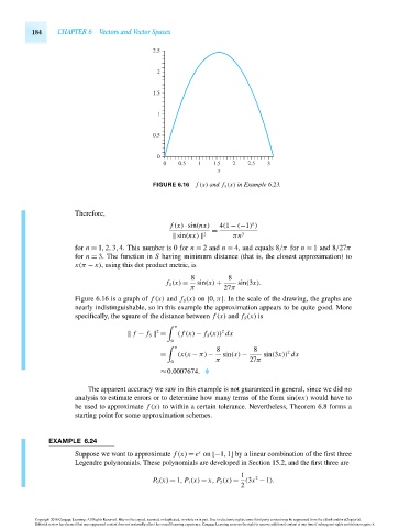
FIGURE 6.16 f (x) and f S (x) in Example 6.23.

Therefore,
n
f (x) · sin(nx) 4(1 − (−1) )
=
sin(nx) 2 πn 3
for n = 1,2,3,4. This number is 0 for n = 2 and n = 4, and equals 8/π for n = 1 and 8/27π
for n = 3. The function in S having minimum distance (that is, the closest approximation) to
x(π − x), using this dot product metric, is
8 8
f S (x) = sin(x) + sin(3x).
π 27π
Figure 6.16 is a graph of f (x) and f S (x) on [0,π]. In the scale of the drawing, the graphs are
nearly indistinguishable, so in this example the approximation appears to be quite good. More
specifically, the square of the distance between f (x) and f S (x) is
π
2 2
f − f S = ( f (x) − f S (x)) dx
0
8 8
π
2
= (x(x − π) − sin(x) − sin(3x)) dx
π 27π
0
≈ 0.0007674.
The apparent accuracy we saw in this example is not guaranteed in general, since we did no
analysis to estimate errors or to determine how many terms of the form sin(nx) would have to
be used to approximate f (x) to within a certain tolerance. Nevertheless, Theorem 6.8 forms a
starting point for some approximation schemes.

EXAMPLE 6.24
x
Suppose we want to approximate f (x) = e on [−1,1] by a linear combination of the first three
Legendre polynomials. These polynomials are developed in Section 15.2, and the first three are
1
2
P 0 (x) = 1, P 1 (x) = x, P 2 (x) = (3x − 1).
2

Copyright 2010 Cengage Learning. All Rights Reserved. May not be copied, scanned, or duplicated, in whole or in part. Due to electronic rights, some third party content may be suppressed from the eBook and/or eChapter(s).
Editorial review has deemed that any suppressed content does not materially affect the overall learning experience. Cengage Learning reserves the right to remove additional content at any time if subsequent rights restrictions require it.

October 14, 2010 14:21 THM/NEIL Page-184 27410_06_ch06_p145-186