Page 246 - Advances in Biomechanics and Tissue Regeneration

242 12. BIOMECHANICAL STUDY IN THE CALCANEUS BONE AFTER AN AUTOLOGOUS BONE HARVEST

12.2 METHODS

The methodology used was a 3-D FE model [15] (Fig. 12.1) that was created based on computed tomography (CT)
images obtained from a healthy male volunteer (36years old, 169-cm height, and 69-kg weight) with no foot pain or
deformities. Twenty-eight foot bones were incorporated into the 3-D model: talus, calcaneus, cuboid, navicular, three
wedges, five metatarsals, five proximal phalanges, four middle phalanges, five phalanges, and two sesamoids. This
model also included the following ligaments: posterior talocalcaneal, calcaneus, navicular, tarsometatarsal, interme-
tatarsal, Lisfranc, calcaneal cuboid–calcaneus–navicular, plantar, and the plantar fascia.
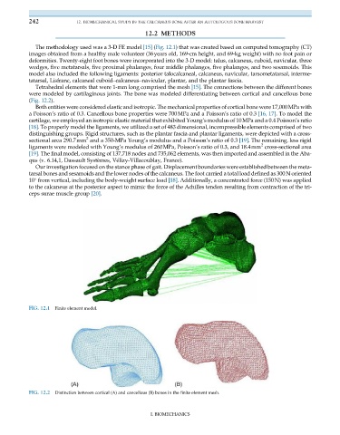
Tetrahedral elements that were 1-mm long comprised the mesh [15]. The connections between the different bones
were modeled by cartilaginous joints. The bone was modeled differentiating between cortical and cancellous bone
(Fig. 12.2).
Both entities were considered elastic and isotropic. The mechanical properties of cortical bone were 17,000MPa with
a Poisson’s ratio of 0.3. Cancellous bone properties were 700MPa and a Poisson’s ratio of 0.3 [16, 17]. To model the
cartilage, we employed an isotropic elastic material that exhibited Young’s modulus of 10MPa and a 0.4 Poisson’s ratio
[18]. To properly model the ligaments, we utilized a set of 483 dimensional, incompressible elements comprised of two
distinguishing groups. Rigid structures, such as the plantar fascia and plantar ligaments, were depicted with a cross-
2
sectional area 290.7mm and a 350-MPa Young’s modulus and a Poisson’s ratio of 0.3 [19]. The remaining, less rigid
2
ligaments were modeled with Young’s modulus of 260MPa, Poisson’s ratio of 0.3, and 18.4mm cross-sectional area
[19]. The final model, consisting of 137,718 nodes and 735,062 elements, was then imported and assembled in the Aba-
qus (v. 6.14,1, Dassault Systèmes, V elizy-Villacoublay, France).
Our investigation focused on the stance phase of gait. Displacement boundaries were established between the meta-
tarsal bones and sesamoids and the lower nodes of the calcaneus. The foot carried a total load defined as 300N oriented
10° from vertical, including the body-weight surface load [18]. Additionally, a concentrated force (150N) was applied
to the calcaneus at the posterior aspect to mimic the force of the Achilles tendon resulting from contraction of the tri-
ceps surae muscle group [20].

FIG. 12.1 Finite element model.

FIG. 12.2 Distinction between cortical (A) and cancellous (B) bones in the finite element mesh.

I. BIOMECHANICS