Page 134 - Aerodynamics for Engineering Students

Potential flow 1 17

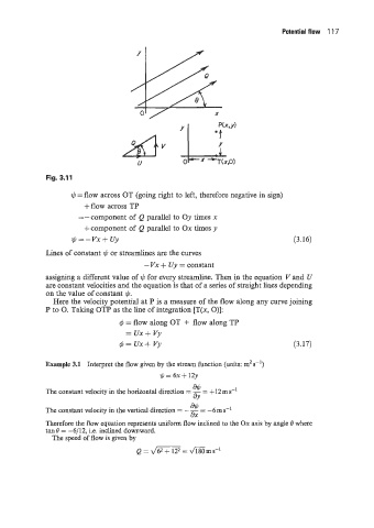
Fig. 3.11

$ = flow across OT (going right to left, therefore negative in sign)
+flow across TP
=-component of Q parallel to Oy times x
+component of Q parallel to Ox times y
$=-vx+ uy (3.16)
Lines of constant $ or streamlines are the curves
-Vx + Uy = constant
assigning a different value of $ for every streamline. Then in the equation V and U
are constant velocities and the equation is that of a series of straight lines depending
on the value of constant $.
Here the velocity potential at P is a measure of the flow along any curve joining
P to 0. Taking OTP as the line of integration [T(x, O)]:

4 = flow along OT + flow along TP
= ux+ vy
c$=vx+vy (3.17)

Example 3.1 Interpret the flow given by the stream function (units: mz s-')
$=6~+12y
w
The constant velocity in the horizontal direction = - = +12rns-'
dY
w
The constant velocity in the vertical direction = - - = -6 m s-]
dX
Therefore the flow equation represents uniform flow inclined to the Ox axis by angle 0 where
tan0 = -6/12, i.e. inclined downward.
The speed of flow is given by
Q = &TiF = mms-'