Page 136 - Aerodynamics for Engineering Students

Potential flow 1 19

Figure 3.12~ shows the flow in the cross-section of a vortex lying parallel to the axis
of a circular duct. The circular duct wall can be replaced by the corresponding
streamline in the vortex-pair system given by the original vortex €3 and its image B'.
It can easily be shown that B' is a distance ?-1s from the centre of the duct on the
diameter produced passing through B, where r is the radius of the duct and s is the
distance of the vortex axis from the centre of the duct.
More complicated contours require more complicated image systems and these are
left until discussion of the cases in which they arise. It will be seen that Fig. 3.12a, which
is the flow of Section 3.3.7, has an internal image system, the source being the image of a
source at --x and the sink being the image of a sink at f-x. This external source and
sink combination produces the undisturbed uniform stream as has been noted above.

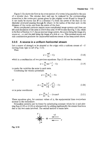
3.3.5 A source in a uniform horizontal stream

Let a source of strength m be situated at the origin with a uniform stream of -U
moving from right to left (Fig. 3.13).
Then
me
$=--uy (3.18)
2n
which is a combination of two previous equations. Eqn (3.18) can be rewritten
m
$=-tan -lY (3.19)
--Uy
2T X
to make the variables the same in each term.
Combining the velocity potentials:
m r
+=-ln--Ux
2n ro
or
5 c; :;)
+=-ln -+- -Ux (3.20)

or in polar coordinates
(3.21)

These equations give, for constant values of +, the equipotential lines everywhere
normal to the streamlines.
Streamline patterns can be found by substituting constant values for $ and plot-
ting Eqn (3.18) or (3.19) or alternatively by adding algebraically the stream functions
due to the two cases involved. The second method is easier here.

Fig. 3.13