Page 165 - Aerodynamics for Engineering Students

148 Aerodynamics for Engineering Students

P

P

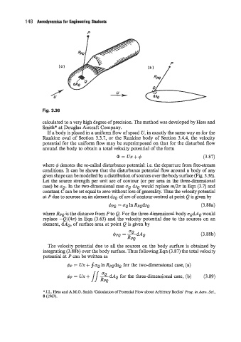
Fig. 3.36

calculated to a very high degree of precision. The method was developed by Hess and
Smith* at Douglas Aircraft Company.
If a body is placed in a uniform flow of speed U, in exactly the same way as for the
Rankine oval of Section 3.3.7, or the Rankine body of Section 3.4.4, the velocity
potential for the uniform flow may be superimposed on that for the disturbed flow
around the body to obtain a total velocity potential of the form
@=Ux++ (3.87)
where + denotes the so-called disturbance potential: i.e. the departure from fresstream
conditions. It can be shown that the disturbance potential flow around a body of any
given shape can be modelled by a distribution of sources over the body surface (Fig. 3.36).
Let the source strength per unit arc of contour (or per area in the three-dimensional
case) be ‘TQ. In the two-dimensional case ‘TQ dsQ would replace m/2~ h Eqn (3.7) and
constant C can be set equal to zero without loss of generality. Thus the velocity potential
at P due to sources on an element dSQ of arc of contour centred at point Q is given by

+PQ = UQ In RPQ~Q (3.8 8a)
where RPQ is the distance from P to Q. For the three-dimensional body ‘TQ~AQ would
replace -Q/(~T) in Eqn (3.63) and the velocity potential due to the sources on an
element, ~AQ, of surface area at point Q is given by

(3.8 8b)

The velocity potential due to all the sources on the body surface is obtained by
integrating (3.88b) over the body surface. Thus following Eqn (3.87) the total velocity
potential at P can be written as
+p = Ux + $‘TQ In RpQdSQ for the two-dimensional case, (a)

+p = Ux + /IPdAQ for the three-dimensional case, (b) (3.89)
RPQ

* J.L. Hess and A.M.O. Smith ‘Calculation of Potential Flow about Arbitrary Bodies’ Prog. in Aero. Sci.,
8 (1967).