Page 168 - Aerodynamics for Engineering Students

Potential flow 151

The calculation of the influence coefficient is a central and essential part of the panel method,
and this is the question now addressed. As a first step consider the calculation of the velocity
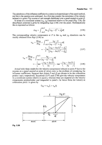
induced at a point P by sources of unit strength distributed over a panel centred at point Q.
In terms of a coordinate system (XQ, YQ) measured relative to the panel (Fig. 3.38), the
disturbance potential is given by integrating Eqn (3.88) over the panel. Mathematically
this is expressed as follows
QPQ = /&I2 In &=iiG&< (3.96)
-&I2
The corresponding velocity components at P in the XQ and YQ directions can be
readily obtained from Eqn (3.96) as

(3.97)

dJ
yQ
(XQ - <)2 + &
= - lm-1 (XO :,”’”> tan-’ ( XQ - yQ AS/^ )]
-
(3.98)

Armed with these results for the velocity components induced at point P due to the
sources on a panel centred at point Q return now to the problem of calculating the
influence coefficients. Suppose that points P and Q are chosen to be the collocation
points i and j respectively. Equations (3.97) and (3.98) give the velocity components
in a coordinate system relative to panel j, whereas what are required are the velocity
components perpendicular and tangential to panel i. In vector form the velocity at
collocation point i is given by

Fig. 3.38