Page 214 - Aerodynamics for Engineering Students

Two-dimensional wing theory 197

and thus Eqn (4.42) is obtained:

This last integral equation relates the chordwise loading, i.e. the vorticity, to the
shape and incidence of the thin aerofoil and by the insertion of a suitable series
expression for k in the integral is capable of solution for both the direct and indirect
aerofoil problems. The aerofoil is reduced to what is in essence a thin lifting sheet,
infinitely long in span, and is replaced by a distribution of singularities that satisfies
the same conditions at the boundaries of the aerofoil system, i.e. at the surface and at
infinity. Further, the theory is a linearized theory that permits, for example, the
velocity at a point in the vicinity of the aerofoil to be taken to be the sum of the
velocity components due to the various characteristics of the system. each treated
separately. As shown in Section 4.3, these linearization assumptions permit an
extension to the theory by allowing a perturbation velocity contribution due to
thickness to be added to the other effects.

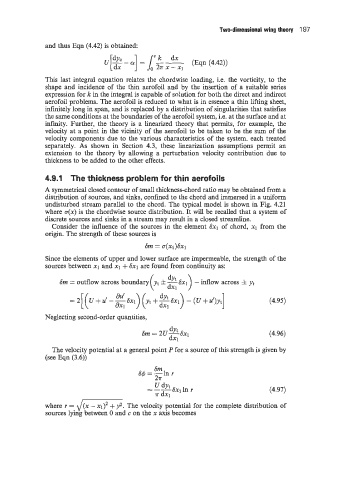
4.9.1 The thickness problem for thin aerofoils
A symmetrical closed contour of small thickness-chord ratio may be obtained from a
distribution of sources, and sinks, confined to the chord and immersed in a uniform
undisturbed stream parallel to the chord. The typical model is shown in Fig. 4.21
where a(x) is the chordwise source distribution. It will be recalled that a system of
discrete sources and sinks in a stream may result in a closed streamline.
Consider the influence of the sources in the element 6x1 of chord, x1 from the
origin. The strength of these sources is
Srn = a(x1)Sxl
Since the elements of upper and lower surface are impermeable, the strength of the
sources between x1 and x1 + 6x1 are found from continuity as:

Sm = outflow across boundary - inflow across f yt

(4.95)

Neglecting second-order quantities,

dYt
Srn = 2U-Sxl (4.96)
dXl
The velocity potential at a general point P for a source of this strength is given by
(see Eqn (3.6))

(4.97)

where r = d(x - xl)’ + y2. The velocity potential for the complete distribution of
sources lying between 0 and c on the x axis becomes